
Model Matrices
In order to introduce model matrices let us start with an example. Five observers test in two conditions. Of theoretical interest is whether the location parameter of the psychometric
function (α, often referred to as 'the threshold') is affected by whatever the experimental manipulation is between the two conditions. Below are (some of the) data from
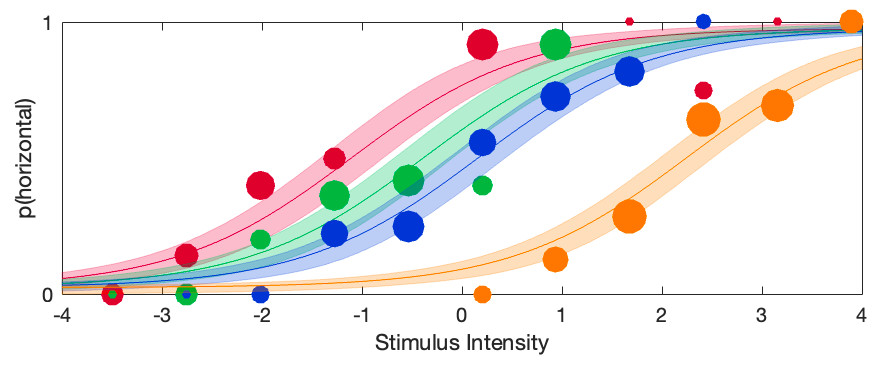
(Prins, Behavior Research Methods, 2024). Each panel shows the data and fits for one observer in two experimental conditions.
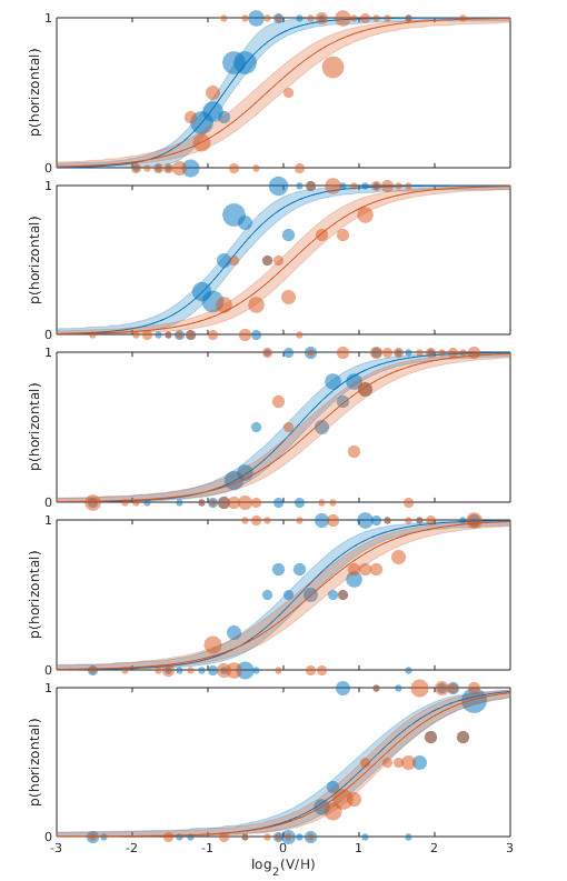 Figure 1. Each panel shows data from one observer testing under two experimental conditions with fits.
By visual inspection of Figure 1, it certainly seems like the location parameter is affected by the manipulation between the two conditions: For all 5 observers the PF for the 'red' condition
is shifted to the right relative to the 'blue' condition, although for some observers the effect is stronger compared to other observers. But when we analyze this with a Hierarchical Bayesian
model (using PAL_PFHB_fitModel), then ask for the violin plots for the mean location parameters in the two conditions:
>> pfhb = PAL_PFHB_fitModel(data,'gammaEQlambda',true,'prior','l','beta',[0.03 100]);
Figure 1. Each panel shows data from one observer testing under two experimental conditions with fits.
By visual inspection of Figure 1, it certainly seems like the location parameter is affected by the manipulation between the two conditions: For all 5 observers the PF for the 'red' condition
is shifted to the right relative to the 'blue' condition, although for some observers the effect is stronger compared to other observers. But when we analyze this with a Hierarchical Bayesian
model (using PAL_PFHB_fitModel), then ask for the violin plots for the mean location parameters in the two conditions:
>> pfhb = PAL_PFHB_fitModel(data,'gammaEQlambda',true,'prior','l','beta',[0.03 100]);
>> PAL_PFHB_drawViolins(pfhb,'amu'); %amu is hyperparameter for location ('threshold') parameter
we get this: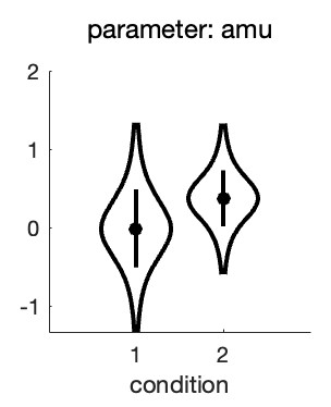 Figure 2. Hyperparameters corresponding to the mean location hyperparameter for both conditions in the experiment
From this, it seems there is very little evidence that the location parameters differ between the conditions! This is not what we were expecting based on our visual inspection of the fitted PFs.
What is happening here is not that the analysis or the violin plot is incorrect, rather the results simply do not correspond to exactly what we are interested in. The violin plot shows the
posteriors for the location hyperparameters in the two conditions. Note however, that when we tried to gauge the experimental effect by visual inspection of Figure 1, we did this not by
estimating the mean location parameter across observers in the 'red' condition and the mean location parameter in the 'blue' condition and comparing those means. Instead we noted that
for each observer individually the red condition was shifted to the right relative to the blue condition. In other words: In our head, we estimated an effect of the manipulation for each observer
individually, then averaged those. In yet other words: When judging the effect, we completely disregarded the fact that the location parameters differed quite a bit between observers. This was
pretty smart of us, because that variance is not relevant to the question of whether location parameters are affected by condition. The problem with the estimates in Figure 2 is that these do not
disregard the differences between average location parameters between observers. This results in the large uncertainty (i.e., wide posteriors) on the estimates.
To give a simple (but unrealistic) analogy, imagine somebody invents a 'smart pill' that is supposed to increase the IQ of whoever takes it. In order to test whether it works, the inventor of the
smart pill finds five willing participants, measures their IQ both before and after taking the smart pill. The results are below:
Figure 2. Hyperparameters corresponding to the mean location hyperparameter for both conditions in the experiment
From this, it seems there is very little evidence that the location parameters differ between the conditions! This is not what we were expecting based on our visual inspection of the fitted PFs.
What is happening here is not that the analysis or the violin plot is incorrect, rather the results simply do not correspond to exactly what we are interested in. The violin plot shows the
posteriors for the location hyperparameters in the two conditions. Note however, that when we tried to gauge the experimental effect by visual inspection of Figure 1, we did this not by
estimating the mean location parameter across observers in the 'red' condition and the mean location parameter in the 'blue' condition and comparing those means. Instead we noted that
for each observer individually the red condition was shifted to the right relative to the blue condition. In other words: In our head, we estimated an effect of the manipulation for each observer
individually, then averaged those. In yet other words: When judging the effect, we completely disregarded the fact that the location parameters differed quite a bit between observers. This was
pretty smart of us, because that variance is not relevant to the question of whether location parameters are affected by condition. The problem with the estimates in Figure 2 is that these do not
disregard the differences between average location parameters between observers. This results in the large uncertainty (i.e., wide posteriors) on the estimates.
To give a simple (but unrealistic) analogy, imagine somebody invents a 'smart pill' that is supposed to increase the IQ of whoever takes it. In order to test whether it works, the inventor of the
smart pill finds five willing participants, measures their IQ both before and after taking the smart pill. The results are below:
 Table 1.
It seems there is quite a bit of evidence that the smart pill works: All of the participants tested higher after the smart pill compared to before. Yet when we compare the difference between
the 'Before' and 'After' means relative to their standard errors we are hardly impressed. The problem is that the SEs for the 'Before' and 'After' means include the differences that participants
brought to the experiment that have nothing to do with how well the smart pill works. Some participants were much smarter than others. This example is similar to the scenario above
because here too we are not interested in how smart these participants were before or how smart they were after. Instead we are interested in whether they got smarter. So we do what
we were taught to do in our introductory statistics course: We reparameterize the model. You might think: I have taken an introductory statistics course but they never taught me to
reparameterize anything, they taught me to do a dependent-samples t-test here! Potato-Potahto. In a dependent-samples t-test the first thing to do is to calculate difference scores, either
'After' - 'Before' or vice versa.
If we do that, the data become:
Table 1.
It seems there is quite a bit of evidence that the smart pill works: All of the participants tested higher after the smart pill compared to before. Yet when we compare the difference between
the 'Before' and 'After' means relative to their standard errors we are hardly impressed. The problem is that the SEs for the 'Before' and 'After' means include the differences that participants
brought to the experiment that have nothing to do with how well the smart pill works. Some participants were much smarter than others. This example is similar to the scenario above
because here too we are not interested in how smart these participants were before or how smart they were after. Instead we are interested in whether they got smarter. So we do what
we were taught to do in our introductory statistics course: We reparameterize the model. You might think: I have taken an introductory statistics course but they never taught me to
reparameterize anything, they taught me to do a dependent-samples t-test here! Potato-Potahto. In a dependent-samples t-test the first thing to do is to calculate difference scores, either
'After' - 'Before' or vice versa.
If we do that, the data become:
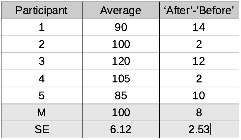 Table 2.
Note that besides calculating the difference scores, we also calculated the average IQ for each participant (i.e., (Before + After)/2) even though these averages are not at all used in a
dependent-samples t-test as they do not tell us anything about how much difference the smart pill makes. We have reparameterized the model. No information was lost when
we did this. From these raparameterized data, we can still figure out what the IQ score of each participant was before and after the smart pill. We will not analyze the 'raw' IQs of participants
or the means of these IQs. Instead we will analyze the reparameterized data, specifically the difference scores. We see that the mean of these improvement scores is 8 points and the
standard error on that number is 2.53. So this would lend much more credibility to the idea that the pill increases IQ.
We need to have Palamedes do the same: Estimate for each observer individually what the effect was of the condition on the PF's location parameter and also estimate the mean of those
effects across participants, complete with posterior and credible intervals and all that. Or means and SEs and p-values if going the frequentist route. Reparameterization works for either.
That means we need to reparameterize the model: Instead of estimating location parameters for condition 1 and location parameters for condition 2, we will estimate, for each observer, the
average location across the two conditions but, of greater theoretical interest, also the difference in locations between the conditions.
We can instruct Palamedes to do this using a model matrix. Model matrices specify new reparameterized parameters (for the sake of convenience, henceforth reparameters) as
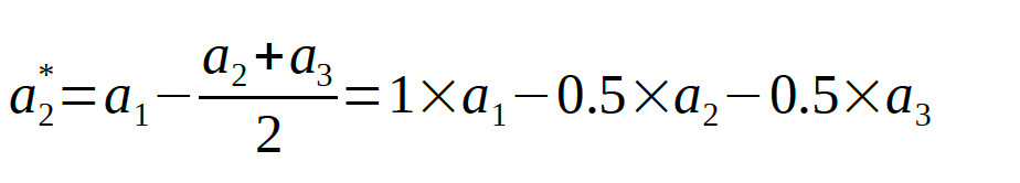
linear combinations of the raw parameters. If we symbolize the location parameters in condition 1 and condition 2 as a1 and a2 respectively, the average
location parameter, of course, is:
Table 2.
Note that besides calculating the difference scores, we also calculated the average IQ for each participant (i.e., (Before + After)/2) even though these averages are not at all used in a
dependent-samples t-test as they do not tell us anything about how much difference the smart pill makes. We have reparameterized the model. No information was lost when
we did this. From these raparameterized data, we can still figure out what the IQ score of each participant was before and after the smart pill. We will not analyze the 'raw' IQs of participants
or the means of these IQs. Instead we will analyze the reparameterized data, specifically the difference scores. We see that the mean of these improvement scores is 8 points and the
standard error on that number is 2.53. So this would lend much more credibility to the idea that the pill increases IQ.
We need to have Palamedes do the same: Estimate for each observer individually what the effect was of the condition on the PF's location parameter and also estimate the mean of those
effects across participants, complete with posterior and credible intervals and all that. Or means and SEs and p-values if going the frequentist route. Reparameterization works for either.
That means we need to reparameterize the model: Instead of estimating location parameters for condition 1 and location parameters for condition 2, we will estimate, for each observer, the
average location across the two conditions but, of greater theoretical interest, also the difference in locations between the conditions.
We can instruct Palamedes to do this using a model matrix. Model matrices specify new reparameterized parameters (for the sake of convenience, henceforth reparameters) as
linear combinations of the raw parameters. If we symbolize the location parameters in condition 1 and condition 2 as a1 and a2 respectively, the average
location parameter, of course, is:
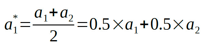 and the diference between location parameters is:
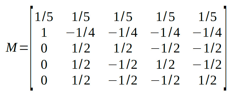
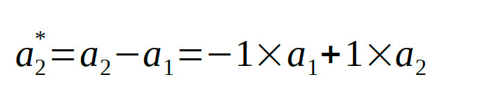 The model matrix that accomplishes the reparameterization simply contains the coefficients of these equations:
 The model matrix has as many columns as there are conditions in the experiment. It has one row for each reparameter we want to estimate. Each row contains the coefficients to use in
the equations specifying the reparameter. Let us analyze these data again, but now estimating the reparameters defined by M instead of the raw location parameters:
>> pfhb = PAL_PFHB_fitModel(data,'gammaEQlambda',true,'prior','l','beta',[0.03 100],'a',M);
The model matrix has as many columns as there are conditions in the experiment. It has one row for each reparameter we want to estimate. Each row contains the coefficients to use in
the equations specifying the reparameter. Let us analyze these data again, but now estimating the reparameters defined by M instead of the raw location parameters:
>> pfhb = PAL_PFHB_fitModel(data,'gammaEQlambda',true,'prior','l','beta',[0.03 100],'a',M);
>> PAL_PFHB_drawViolins(pfhb,'amu');
which gives: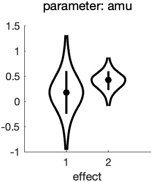 Figure 3. Hyperparameters corresponding to the mean location hyperreparameters
Note that the x-axis now is labeled 'effect' and not 'condition' (as was the case in Figure 2). This is because the parameters represented in the figure no longer correspond to the location
parameters for each condition, but instead correspond to the reparameters: the mean and the difference, respectively, of the location parameters.
A few things to note from the violin plot: the mean parameter ('effect 1') has much more uncertainty associated with it compared to the difference parameter ('effect 2'). This is because the
observers differed quite a bit with respect to the average location of the PFs (see Figure 1). Much more so than they did with respect to the difference between the two PF locations.
Of theoretical interest, it is now clear that a value of zero is not very credible for the mean of the difference parameter (effect 2). This corresponds with our idea about the effect of
condition based on our casual inspection of Figure 1.
Note that even though we are not really interested in the average location of the PFs (i.e., a1*), leaving it out of the Model Matrix means that Palamedes would leave this 'effect' out of the model,
which effectively means that the model would be forced to keep the average location parameters (a1*) at 0, which would make for a very poor model. Note that we have reparameterized two
parameters (one location parameter for each of the two conditions) into two new reparameters (the average and difference between the two location parameters). Importantly,
these reparameterizations defined in the model matrix are orthogonal. In plain English, this means that each reparameter affects things that the other parameter has no control
over whatsoever. The value of a1* affects the average location parameter across conditions but does not affect the difference between the location
parameters whatsoever. Conversely, the value of a2* affects the difference between location parameters across conditions but does not affect the
average location parameters whatsoever. Whenever you reparameterize n parameters into n new parameters that are all mutually orthogonal, the reparameterized model is not constrained
in any way relative to the original model1. It is easy to verify whether two reparameters are orthogonal using the model matrix: Multiply the coefficients across the two rows,
then sum these products. If the sum equals 0, the parameters are orthogonal. Visually:
Figure 3. Hyperparameters corresponding to the mean location hyperreparameters
Note that the x-axis now is labeled 'effect' and not 'condition' (as was the case in Figure 2). This is because the parameters represented in the figure no longer correspond to the location
parameters for each condition, but instead correspond to the reparameters: the mean and the difference, respectively, of the location parameters.
A few things to note from the violin plot: the mean parameter ('effect 1') has much more uncertainty associated with it compared to the difference parameter ('effect 2'). This is because the
observers differed quite a bit with respect to the average location of the PFs (see Figure 1). Much more so than they did with respect to the difference between the two PF locations.
Of theoretical interest, it is now clear that a value of zero is not very credible for the mean of the difference parameter (effect 2). This corresponds with our idea about the effect of
condition based on our casual inspection of Figure 1.
Note that even though we are not really interested in the average location of the PFs (i.e., a1*), leaving it out of the Model Matrix means that Palamedes would leave this 'effect' out of the model,
which effectively means that the model would be forced to keep the average location parameters (a1*) at 0, which would make for a very poor model. Note that we have reparameterized two
parameters (one location parameter for each of the two conditions) into two new reparameters (the average and difference between the two location parameters). Importantly,
these reparameterizations defined in the model matrix are orthogonal. In plain English, this means that each reparameter affects things that the other parameter has no control
over whatsoever. The value of a1* affects the average location parameter across conditions but does not affect the difference between the location
parameters whatsoever. Conversely, the value of a2* affects the difference between location parameters across conditions but does not affect the
average location parameters whatsoever. Whenever you reparameterize n parameters into n new parameters that are all mutually orthogonal, the reparameterized model is not constrained
in any way relative to the original model1. It is easy to verify whether two reparameters are orthogonal using the model matrix: Multiply the coefficients across the two rows,
then sum these products. If the sum equals 0, the parameters are orthogonal. Visually:
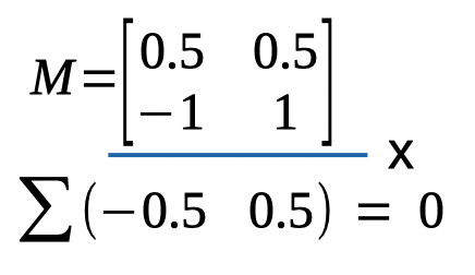 Figure 4. Verifying orthogonality of reparameterizations
The sum of the products indeed equals zero, confirming that the two reparameterizations are orthogonal. Having verified the two conditions above (we have as many reparameters as we had
'raw' parameters and the reparameterizations are orthogonal), we can rest assured that our reparameterization does not restrict our new model relative to its original parameterization.
Note that it can be useful to restrict a model. Remember that more parameters does not necessarily make for a better model. It can be useful to restrict (or constrain) the model that
Palamedes can fit by leaving effects out of the Model Matrix. As a matter of fact, the fit performed above used the Model Matrix [0.5 0.5] for the lapse rate parameter. In other words,
the model estimated only the average lapse rate between the two conditions and thereby did not allow for a difference between conditions. Effectively, this means that the model assumes
that the actual generating lapse rate was equal across conditions (but could still differ between observers). This would, generally speaking, be a sensible assumption that makes for a better
model (see Prins, 2024).
Leaving effects out of the model also allows a comparison between two versions of a model: One which includes the effect and one which does not. One could then compare the fit of the
two models using, for example, one of the information criteria (AIC, BIC, etc.). In the above example, one could compare the fit of a model that includes both
a1* and a2* (the difference parameter)
to one that includes only a1*. The former would allow the location parameters to differ, the latter would not.
It is perfectly fine to use different parameterizations for the different parameters of the PF. Above, we reparameterized the location parameter into the average location and the difference
between locations. We used a different reparameterization for the lapse rate in order to constrain the lapse rates to be equal between conditions. Finally, we did not reparameterize the slope parameters at all.
Figure 4. Verifying orthogonality of reparameterizations
The sum of the products indeed equals zero, confirming that the two reparameterizations are orthogonal. Having verified the two conditions above (we have as many reparameters as we had
'raw' parameters and the reparameterizations are orthogonal), we can rest assured that our reparameterization does not restrict our new model relative to its original parameterization.
Note that it can be useful to restrict a model. Remember that more parameters does not necessarily make for a better model. It can be useful to restrict (or constrain) the model that
Palamedes can fit by leaving effects out of the Model Matrix. As a matter of fact, the fit performed above used the Model Matrix [0.5 0.5] for the lapse rate parameter. In other words,
the model estimated only the average lapse rate between the two conditions and thereby did not allow for a difference between conditions. Effectively, this means that the model assumes
that the actual generating lapse rate was equal across conditions (but could still differ between observers). This would, generally speaking, be a sensible assumption that makes for a better
model (see Prins, 2024).
Leaving effects out of the model also allows a comparison between two versions of a model: One which includes the effect and one which does not. One could then compare the fit of the
two models using, for example, one of the information criteria (AIC, BIC, etc.). In the above example, one could compare the fit of a model that includes both
a1* and a2* (the difference parameter)
to one that includes only a1*. The former would allow the location parameters to differ, the latter would not.
It is perfectly fine to use different parameterizations for the different parameters of the PF. Above, we reparameterized the location parameter into the average location and the difference
between locations. We used a different reparameterization for the lapse rate in order to constrain the lapse rates to be equal between conditions. Finally, we did not reparameterize the slope parameters at all.
 The reparameters are identical to the raw parameters, i.e., the identity matrix doesn't really
reparameterize your model at all. In Palamedes fitting routines, the identity matrix is the default for the location and slope parameters of a PF.
The reparameters are identical to the raw parameters, i.e., the identity matrix doesn't really
reparameterize your model at all. In Palamedes fitting routines, the identity matrix is the default for the location and slope parameters of a PF.
 So the corresponding row in the Model Matrix will be:
[1 -0.5 -0.5]
Note that the coefficients in the row add to zero. This is a good thing. If the coefficients add to zero, the row will be orthogonal to the first row (which defined the average). If the coefficients
do not add to zero, the row will not be orthogonal to the first row.
The second Helmert contrast compares the two conditions that were grouped together in the first Helmert contrast (i.e., conditions 2 and 3) against each other:
[0 1 -1]
Thus, the full model matrix is:
So the corresponding row in the Model Matrix will be:
[1 -0.5 -0.5]
Note that the coefficients in the row add to zero. This is a good thing. If the coefficients add to zero, the row will be orthogonal to the first row (which defined the average). If the coefficients
do not add to zero, the row will not be orthogonal to the first row.
The second Helmert contrast compares the two conditions that were grouped together in the first Helmert contrast (i.e., conditions 2 and 3) against each other:
[0 1 -1]
Thus, the full model matrix is:
 We leave it to the reader to verify that all pairs of rows in the matrix are mutually orthogonal.
The Palamedes routine PAL_Contrasts can generate a model matrix containing Helmert contrasts:
>>M = PAL_Contrasts(3,'Helmert') %type help PAL_Contrasts for details on use
We leave it to the reader to verify that all pairs of rows in the matrix are mutually orthogonal.
The Palamedes routine PAL_Contrasts can generate a model matrix containing Helmert contrasts:
>>M = PAL_Contrasts(3,'Helmert') %type help PAL_Contrasts for details on use
which gives: M =
1 1 1
2 -1 -1
0 1 -1 Note that each row is actually a multiple of the matrix given above such that all entries are whole numbers. Each row is simply a multiple of the corresponding row in the matrix above. This changes the interpretation of the parameter estimates. For example, in the matrix generated by PAL_Contrasts, the first reparameter corresponds to the sum (rather than the average) across the conditions. In general, we recommend creating model matrices for which the reparameters can be thought of to correspond to averages or differences between averages (e.g., the reparameter defined by the second row corresponds to [1 -0.5 -0.5], that is: 'condition 1 - the average of conditions 2 and 3'). In order to do this, for each row simply divide the coefficients by the sum of the positive coefficients in the row. Multiplying/dividing all coefficients in a row by a constant does not change whether the reparameterization defined by that row is or is not orthogonal with the other reparameterizations in the matrix. Note that the order of conditions is arbitrary, so you can the shuffle the order of the columns around if that makes for more theoretically meaningful comparisons (but the entire column must be shifted, not just columns within individual rows), resulting for example in: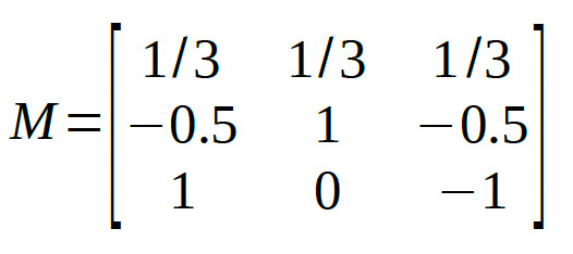
 The violin plots for the raw location parameters look like this:
 It seems clear that the location parameter values generally increase with adaptation duration (that would be the 'linear trend'), but it is less clear whether the bend in the relationship is 'real'
or not (that would be the 'quadratic trend'). A model matrix containing polynomial contrast addresses this question. The function PAL_Contrast can generate a model matrix for a trend
analysis:
>>M = PAL_Contrasts(4,'polynomial') %type help PAL_Contrasts for details on use
It seems clear that the location parameter values generally increase with adaptation duration (that would be the 'linear trend'), but it is less clear whether the bend in the relationship is 'real'
or not (that would be the 'quadratic trend'). A model matrix containing polynomial contrast addresses this question. The function PAL_Contrast can generate a model matrix for a trend
analysis:
>>M = PAL_Contrasts(4,'polynomial') %type help PAL_Contrasts for details on use
which gives: M =
1 1 1 1
-3 -1 1 3
1 -1 -1 1
-1 3 -3 1 These four reparameters are orthogonal. Using this matrix to reparameterize the location parameters, then asking for the violin plots give this: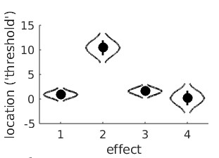 'effect 1' is the reparameter defined by the first row of M, in other words the sum of the four location parameters. The 'effect 2' reparameter is the linear trend. We see that, as expected, it
is likely to have a high, positive value (and that a value of 0 is effectively impossible). This confirms that thresholds indeed tend to rise with adaptation duration. The 'effect 3'
reparameter is the quadratic trend and, simply put, allows the line to have a bend. In this violin plot, the posterior for the quadratic trend is a bit smooshed, but we can create a violin plot for 'effect 3' separately using:
>>PAL_PFHB_drawViolins(pfhb,'effect',3)
'effect 1' is the reparameter defined by the first row of M, in other words the sum of the four location parameters. The 'effect 2' reparameter is the linear trend. We see that, as expected, it
is likely to have a high, positive value (and that a value of 0 is effectively impossible). This confirms that thresholds indeed tend to rise with adaptation duration. The 'effect 3'
reparameter is the quadratic trend and, simply put, allows the line to have a bend. In this violin plot, the posterior for the quadratic trend is a bit smooshed, but we can create a violin plot for 'effect 3' separately using:
>>PAL_PFHB_drawViolins(pfhb,'effect',3)
It is now clear that a value of 0 is not very likely for the quadratic trend which may suggest that the bend is 'real'.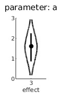
 The full matrix then is:
 We leave it up to the reader to verify that these 6 reparameterizations are indeed all mutually orthogonal.
Note that Helmert contrasts can be formed using a tree diagram. Note also that while any set of contrasts that divides parameters according to a tree diagram will result in a set of
orthogonal contrasts, a set of contrasts may still be orthogonal even in cases where they do not follow a tree diagram. One example of this is the set of polynomial contrasts given above.
Some more examples are discussed below.
We leave it up to the reader to verify that these 6 reparameterizations are indeed all mutually orthogonal.
Note that Helmert contrasts can be formed using a tree diagram. Note also that while any set of contrasts that divides parameters according to a tree diagram will result in a set of
orthogonal contrasts, a set of contrasts may still be orthogonal even in cases where they do not follow a tree diagram. One example of this is the set of polynomial contrasts given above.
Some more examples are discussed below.
 The first reparameter is easy:
As in all examples so far, it corresponds to the average across all conditions. However, for now, we will use only integers for coefficients and we will normalize the coefficients later. Thus
our first row, for now, will be:
[1 1 1 1]
Let's make our second reparameter correspond to the main effect of IV A. Also easy. The reparameter will be the average of conditions under level 1 of A minus the
average of conditions under level 2 of A (but, again for now we will use integers only):
[1 1 -1 -1]
Our third reparameter will correspond to the main effect of IV B. Just as easy as the previous one. The reparameter will be the average of conditions under level 1 of B
minus the average of conditions under level 2 of B (but, again for now we will use integers only):
[1 -1 1 -1]
Our last parameter will correspond to the A × B interaction. Conceptually not as easy as the first three reparameters, but lucky for us, in practice very easy to create. Interaction
reparameters can simply be found by multiplying the coefficients across the main effect reparameterizations (there is a reason interactions are often notated using the
multiplication symbol [e.g., 'A × B'], as we did above!). Thus, our last reparameter is defined by:
[1×1 1×-1 -1×1 -1×-1]
or:
[1 -1 -1 1]
The full matrix:
The first reparameter is easy:
As in all examples so far, it corresponds to the average across all conditions. However, for now, we will use only integers for coefficients and we will normalize the coefficients later. Thus
our first row, for now, will be:
[1 1 1 1]
Let's make our second reparameter correspond to the main effect of IV A. Also easy. The reparameter will be the average of conditions under level 1 of A minus the
average of conditions under level 2 of A (but, again for now we will use integers only):
[1 1 -1 -1]
Our third reparameter will correspond to the main effect of IV B. Just as easy as the previous one. The reparameter will be the average of conditions under level 1 of B
minus the average of conditions under level 2 of B (but, again for now we will use integers only):
[1 -1 1 -1]
Our last parameter will correspond to the A × B interaction. Conceptually not as easy as the first three reparameters, but lucky for us, in practice very easy to create. Interaction
reparameters can simply be found by multiplying the coefficients across the main effect reparameterizations (there is a reason interactions are often notated using the
multiplication symbol [e.g., 'A × B'], as we did above!). Thus, our last reparameter is defined by:
[1×1 1×-1 -1×1 -1×-1]
or:
[1 -1 -1 1]
The full matrix:
 The four reparameters are all mutually orthogonal. As a last step, let's normalize the matrix such that the reparameters can be interpreted as averages or differences
between averages (this will not change whether rows are orthogonal):
The four reparameters are all mutually orthogonal. As a last step, let's normalize the matrix such that the reparameters can be interpreted as averages or differences
between averages (this will not change whether rows are orthogonal):
 At first glance, the interaction contrast might not make much sense. Let's take a look at the non-normalized coefficients:
[1 -1 -1 1]
Thus the interaction reparameter is defined as:
A1B1 - A1B2 - A2B1 + A2B2
(where e.g., A1B2 refers to the condition that is under level 1 of Factor A and level 2 of Factor B)
In order to see that this indeed corresponds to the interaction of the two Factors note that this is equivalent to
(A2B2-A2B1)-(A1B2-A1B1)
The term within the first set of parentheses (i.e., A2B2 - A2B1) is the effect that IV B has within the second level of IV A. The term within the second set of parentheses (i.e., A1B2 - A1B1)
is the effect IV B has within the first level of IV A. Thus, when the effect of B is the same in both levels of A
(i.e., Factor A and Factor B do not interact), the interaction reparameter equals 0. If the effect of B differs
between the two levels of A (i.e., Factor A and Factor B interact), the reparameter will take on a value other than 0.
Note that this model matrix could not have been created using the tree method above, but nevertheless consists of reparameterizations that are all mutually orthogonal.
2 × 3 Factorial design
Let's say one of your IVs (A) in a factorial design has 2 levels and the other (B) has 3 levels, resulting in 6 conditions (see Table below for a listing of the conditions).
At first glance, the interaction contrast might not make much sense. Let's take a look at the non-normalized coefficients:
[1 -1 -1 1]
Thus the interaction reparameter is defined as:
A1B1 - A1B2 - A2B1 + A2B2
(where e.g., A1B2 refers to the condition that is under level 1 of Factor A and level 2 of Factor B)
In order to see that this indeed corresponds to the interaction of the two Factors note that this is equivalent to
(A2B2-A2B1)-(A1B2-A1B1)
The term within the first set of parentheses (i.e., A2B2 - A2B1) is the effect that IV B has within the second level of IV A. The term within the second set of parentheses (i.e., A1B2 - A1B1)
is the effect IV B has within the first level of IV A. Thus, when the effect of B is the same in both levels of A
(i.e., Factor A and Factor B do not interact), the interaction reparameter equals 0. If the effect of B differs
between the two levels of A (i.e., Factor A and Factor B interact), the reparameter will take on a value other than 0.
Note that this model matrix could not have been created using the tree method above, but nevertheless consists of reparameterizations that are all mutually orthogonal.
2 × 3 Factorial design
Let's say one of your IVs (A) in a factorial design has 2 levels and the other (B) has 3 levels, resulting in 6 conditions (see Table below for a listing of the conditions).
 Let's see if we can find 6 orthogonal reparameters that correspond to the average, the main effects and the interactions. The first reparameter is the average (but
again for now let's stick to integers and actually make it the sum):
[1 1 1 1 1 1]
Next, the main effect of A. It might help here to consider how many degrees of freedom are associated with the main effect for A. From our introductory statistics class we remember
(hopefully) that a factor with two levels has one degree of freedom associated with it. That translates here to needing only 1 reparameter to represent the differences among
the two levels of the factor. The reparameter corresponds to the average across, say, the conditions in the first level of A minus the average across the conditions in the second
level of A. Using the ordering of the 6 conditions shown in the table above, and again sticking to integers for now, the coefficients for the reparameter are:
[1 1 1 -1 -1 -1]
Now for the main effects of factor B. No, the plural 's' in 'effects' is not a typo. Remember that a main effect for an IV with three levels has 2 degrees of freedom, which translates here
as requiring two reparameters to define the main effects for Factor B. It is easier to forget for now about the other Factor and pretend we're designing reparameters
for a simple one-factor experiment where the factor has three levels: B1, B2, and B3. Let's use Helmert contrasts here just like we did way above when we were considering a simple,
one-factor experiment with three levels and used Helmert contrasts. However, we'll stick again to using only integers for now and use:
[2 -1 -1]
and
[0 1 -1]
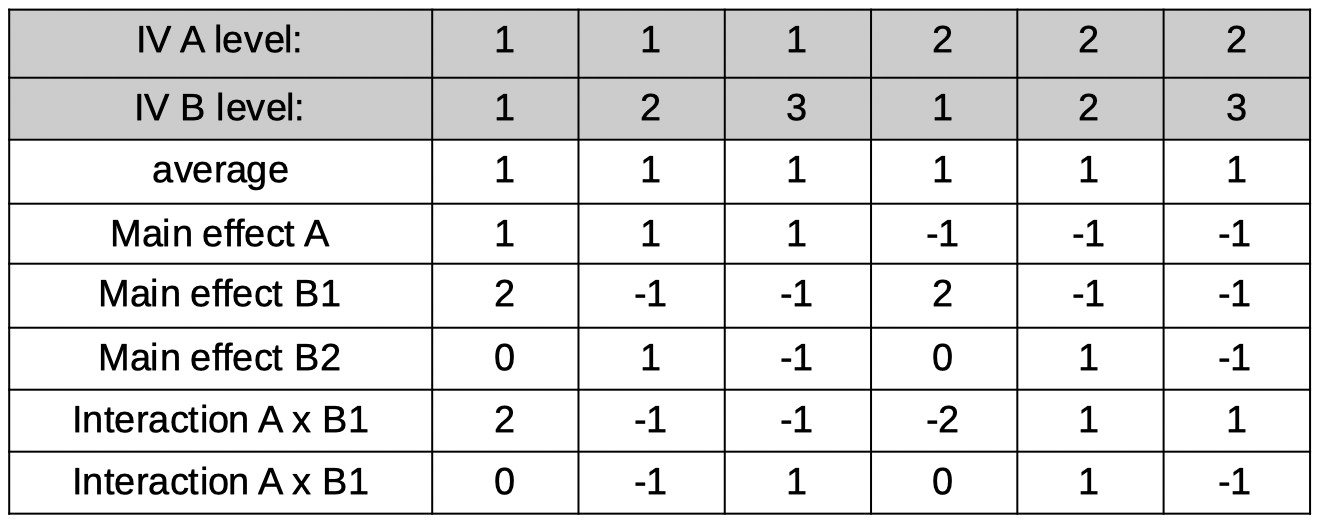
expanding this across all six conditions in our experiment gives the reparameters labeled 'main effect B1' and 'main effect B2' in the table above. Note that we simply made
two copies of the coefficients: One for the conditions under level 1 of A, the other for conditions under level 2 of A.
All that is left is to find the two reparameters that will define the interactions (plural 's' intended!). Note that again, the number of reparameters needed is equal to
the degrees of freedom associated with the effect. In a 2 × 3 the number of degrees of freedom associated with the interaction equals 2. Practically, the coefficients for these are easy
to find. One interaction will be the interaction between the main effect of A and the first main effect on B (labeled B1 above). The coefficients correspond again simply to the products of the two interacting
main effects, so we simply multiply the coefficients in the 'main effect A' row with the coefficients in the 'main effect B1' row. In a similar fashion, we can find the coefficients for the
A × B2 interaction. You may have realized by now that we chose to stick to integer values for coefficients for now because that makes the multiplication of coefficients to find the
interactions much easier. Normalization of the coefficients in the table results in the final model matrix:
Let's see if we can find 6 orthogonal reparameters that correspond to the average, the main effects and the interactions. The first reparameter is the average (but
again for now let's stick to integers and actually make it the sum):
[1 1 1 1 1 1]
Next, the main effect of A. It might help here to consider how many degrees of freedom are associated with the main effect for A. From our introductory statistics class we remember
(hopefully) that a factor with two levels has one degree of freedom associated with it. That translates here to needing only 1 reparameter to represent the differences among
the two levels of the factor. The reparameter corresponds to the average across, say, the conditions in the first level of A minus the average across the conditions in the second
level of A. Using the ordering of the 6 conditions shown in the table above, and again sticking to integers for now, the coefficients for the reparameter are:
[1 1 1 -1 -1 -1]
Now for the main effects of factor B. No, the plural 's' in 'effects' is not a typo. Remember that a main effect for an IV with three levels has 2 degrees of freedom, which translates here
as requiring two reparameters to define the main effects for Factor B. It is easier to forget for now about the other Factor and pretend we're designing reparameters
for a simple one-factor experiment where the factor has three levels: B1, B2, and B3. Let's use Helmert contrasts here just like we did way above when we were considering a simple,
one-factor experiment with three levels and used Helmert contrasts. However, we'll stick again to using only integers for now and use:
[2 -1 -1]
and
[0 1 -1]
expanding this across all six conditions in our experiment gives the reparameters labeled 'main effect B1' and 'main effect B2' in the table above. Note that we simply made
two copies of the coefficients: One for the conditions under level 1 of A, the other for conditions under level 2 of A.
All that is left is to find the two reparameters that will define the interactions (plural 's' intended!). Note that again, the number of reparameters needed is equal to
the degrees of freedom associated with the effect. In a 2 × 3 the number of degrees of freedom associated with the interaction equals 2. Practically, the coefficients for these are easy
to find. One interaction will be the interaction between the main effect of A and the first main effect on B (labeled B1 above). The coefficients correspond again simply to the products of the two interacting
main effects, so we simply multiply the coefficients in the 'main effect A' row with the coefficients in the 'main effect B1' row. In a similar fashion, we can find the coefficients for the
A × B2 interaction. You may have realized by now that we chose to stick to integer values for coefficients for now because that makes the multiplication of coefficients to find the
interactions much easier. Normalization of the coefficients in the table results in the final model matrix:
 As usual, we will leave it up to the reader to verify that all 6 reparameterizations are orthogonal.
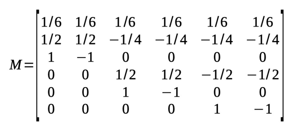
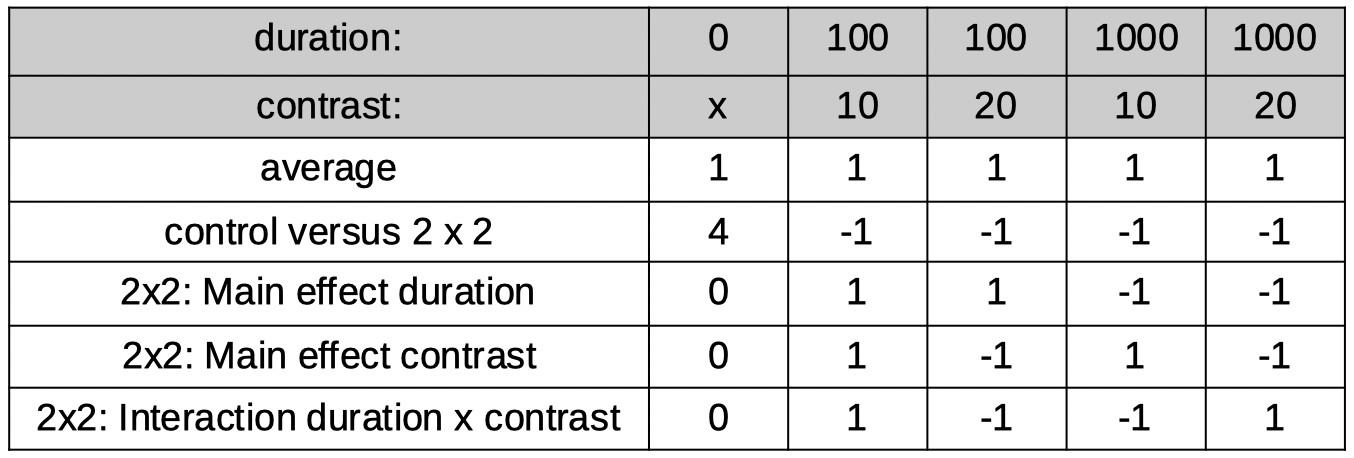 Many different model matrices can be created to reparameterize these 5 conditions into 5 orthogonal reparameters. However, we should create one that isolates interesting
research questions. Let's say we have a specific interest in determining whether duration and contrast interact (when there is in fact an adapting stimulus). So we want one of the 5
reparameters to correspond to that interaction. What we can do to accomplish this is to first use the tree method above to identify a reparameter that separates the 5
conditions into the control condition on the one hand and the 2 × 2 section of the design on the other, then to use the reparameterization for the 2 × 2 design derived above to
reparameterize the 2 × 2 section of the design. The coefficients in the table below do just that.
Normalization of the coefficients leads to:
Many different model matrices can be created to reparameterize these 5 conditions into 5 orthogonal reparameters. However, we should create one that isolates interesting
research questions. Let's say we have a specific interest in determining whether duration and contrast interact (when there is in fact an adapting stimulus). So we want one of the 5
reparameters to correspond to that interaction. What we can do to accomplish this is to first use the tree method above to identify a reparameter that separates the 5
conditions into the control condition on the one hand and the 2 × 2 section of the design on the other, then to use the reparameterization for the 2 × 2 design derived above to
reparameterize the 2 × 2 section of the design. The coefficients in the table below do just that.
Normalization of the coefficients leads to:
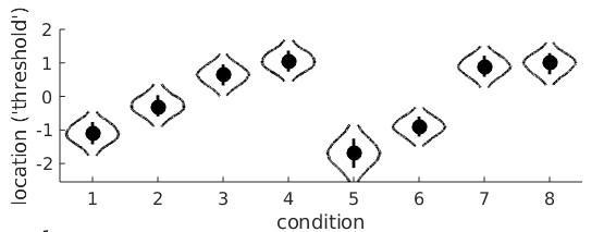 Conditions 1-4 are the monocular conditions, conditions 5-8 are the binocular conditions. It seems clear that there is a linear trend main effect: in both the monocular and binocular
viewing conditions, the location parameters generally increase with adaptation duration. However, it seems that they increase a bit faster in the binocular viewing condition compared
to the monocular conditions. This would be the linear trend on adaptation duration × viewing condition interaction. Let's set up the model matrix. We have 8 raw location parameters, we
would like 8 orthogonal reparameters. This may seem like a difficult task, but it is not. The first one is routine by now. It is the average location:
M(1,:) = [1/8 1/8 1/8 1/8 1/8 1/8 1/8 1/8];
Next, let's work on the main effect of Factor A (monocular versus binocular viewing condition). There are two levels, thus one degree of freedom or one reparameter. Also easy: we'll make it
the sum of the location parameters under binocular viewing minus the sum of the location parameters under the monocular viewing conditions. This is essentially the same 'difference'
reparameter from the very first example above except now it has to be expanded because it is crossed with the second variable. If the order in which the conditions are numbered in the data
structure is A1B1 A1B2 A1B3 A1B4 A2B1 A2B2 A2B3 A2B4 (i.e., conditions are ordered as in the violin plot above) then our second reparameter is:
M(2,:) = [-1 -1 -1 -1 1 1 1 1];
The natural next thing to work on is the main effects of Factor B. Yes, that's again a plural 'effects' because Factor B has 4 levels, 3 degrees of freedoms and thus 3 reparameters that
define the main effects of this Factor. Just like above in the example where adaptation duration was the only factor, we will use polynomial contrasts. But, because of the other Factor, we will need to expand again
to cover both instances of each adaptation duration:
M(3,:) = [-3 -1 1 3 -3 -1 1 3];
M(4,:) = [1 -1 -1 1 1 -1 -1 1];
M(5,:) = [-1 3 -3 1 -1 3 -3 1];
These are the main (as in 'main effect') linear trend on adaptation duration, the main quadratic trend on adaptation duration, and the main cubic trend on adaptation duration, respectively. We have
5 reparameters so far, so we need three more to complete the set. Of course, these will be the interaction effects. Remember that in a 2×4 design there are three degrees of freedom associated with the
interaction and thus three reparameters. We can find these again simply by multiplying contrasts coefficients across the main effects:
M(6,:) = M(2,:).*M(3,);
M(7,:) = M(2,:).*M(4,);
M(8,:) = M(2,:).*M(5,);
These are the viewing condition × linear trend on adaptation duration interaction ('does the general rate of increase of the location parameter differ between monocular and binocular viewing?'),
viewing condition × quadratic trend on adaptation duration interaction ('does the quadratic trend differ between monocular and binocular viewing?'), and the viewing condition × cubic trend on
adaptation duration interaction ('does the cubic trend differ between monocular and binocular viewing), respectively.
That's it. These 8 reparameterizations are all mutually orthogonal (but feel free to check). Analyzing the data again with the reparametrized location parameters gives these violin plots:
Conditions 1-4 are the monocular conditions, conditions 5-8 are the binocular conditions. It seems clear that there is a linear trend main effect: in both the monocular and binocular
viewing conditions, the location parameters generally increase with adaptation duration. However, it seems that they increase a bit faster in the binocular viewing condition compared
to the monocular conditions. This would be the linear trend on adaptation duration × viewing condition interaction. Let's set up the model matrix. We have 8 raw location parameters, we
would like 8 orthogonal reparameters. This may seem like a difficult task, but it is not. The first one is routine by now. It is the average location:
M(1,:) = [1/8 1/8 1/8 1/8 1/8 1/8 1/8 1/8];
Next, let's work on the main effect of Factor A (monocular versus binocular viewing condition). There are two levels, thus one degree of freedom or one reparameter. Also easy: we'll make it
the sum of the location parameters under binocular viewing minus the sum of the location parameters under the monocular viewing conditions. This is essentially the same 'difference'
reparameter from the very first example above except now it has to be expanded because it is crossed with the second variable. If the order in which the conditions are numbered in the data
structure is A1B1 A1B2 A1B3 A1B4 A2B1 A2B2 A2B3 A2B4 (i.e., conditions are ordered as in the violin plot above) then our second reparameter is:
M(2,:) = [-1 -1 -1 -1 1 1 1 1];
The natural next thing to work on is the main effects of Factor B. Yes, that's again a plural 'effects' because Factor B has 4 levels, 3 degrees of freedoms and thus 3 reparameters that
define the main effects of this Factor. Just like above in the example where adaptation duration was the only factor, we will use polynomial contrasts. But, because of the other Factor, we will need to expand again
to cover both instances of each adaptation duration:
M(3,:) = [-3 -1 1 3 -3 -1 1 3];
M(4,:) = [1 -1 -1 1 1 -1 -1 1];
M(5,:) = [-1 3 -3 1 -1 3 -3 1];
These are the main (as in 'main effect') linear trend on adaptation duration, the main quadratic trend on adaptation duration, and the main cubic trend on adaptation duration, respectively. We have
5 reparameters so far, so we need three more to complete the set. Of course, these will be the interaction effects. Remember that in a 2×4 design there are three degrees of freedom associated with the
interaction and thus three reparameters. We can find these again simply by multiplying contrasts coefficients across the main effects:
M(6,:) = M(2,:).*M(3,);
M(7,:) = M(2,:).*M(4,);
M(8,:) = M(2,:).*M(5,);
These are the viewing condition × linear trend on adaptation duration interaction ('does the general rate of increase of the location parameter differ between monocular and binocular viewing?'),
viewing condition × quadratic trend on adaptation duration interaction ('does the quadratic trend differ between monocular and binocular viewing?'), and the viewing condition × cubic trend on
adaptation duration interaction ('does the cubic trend differ between monocular and binocular viewing), respectively.
That's it. These 8 reparameterizations are all mutually orthogonal (but feel free to check). Analyzing the data again with the reparametrized location parameters gives these violin plots:
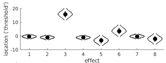 From the violin plot we see that reparameter 3 (main linear trend on adaptation duration) is positive and very unlikely to include 0 confirming that, averaged between monocular and
binocular viewing conditions, the location parameters increase with adaptation duration. We also see that reparameter 6 (viewing condition × linear trend on adaptation duration) is
positive and unlikely to include 0 suggesting that the apparent faster rate of increase of location parameter with adaptation duration when stimuli are viewed binocularly compared to monocularly is 'real'.
From the violin plot we see that reparameter 3 (main linear trend on adaptation duration) is positive and very unlikely to include 0 confirming that, averaged between monocular and
binocular viewing conditions, the location parameters increase with adaptation duration. We also see that reparameter 6 (viewing condition × linear trend on adaptation duration) is
positive and unlikely to include 0 suggesting that the apparent faster rate of increase of location parameter with adaptation duration when stimuli are viewed binocularly compared to monocularly is 'real'.
 You can also constrain model parameters by leaving out any combination of the reparameters from a model matrix. To give one example, in the analysis under 'Polynomial Contrasts' above
we reparameterized the four location parameters into four orthogonal reparameters using polynomial contrasts. Thus, this reparameterization did not constrain the location parameters at all.
We can constrain the location parameters to increase strictly linearly as a function of adaptation duration by including only the first and second rows of the
model matrix (i.e., the 'intercept' and linear trend). thus the model matrix we'll use is:
M =
You can also constrain model parameters by leaving out any combination of the reparameters from a model matrix. To give one example, in the analysis under 'Polynomial Contrasts' above
we reparameterized the four location parameters into four orthogonal reparameters using polynomial contrasts. Thus, this reparameterization did not constrain the location parameters at all.
We can constrain the location parameters to increase strictly linearly as a function of adaptation duration by including only the first and second rows of the
model matrix (i.e., the 'intercept' and linear trend). thus the model matrix we'll use is:
M =
[ 1 1 1 1;
-3 -1 1 3] The fitted psychometric functions looks like this: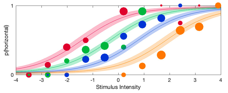 Note that now the location parameters are indeed equally spaced and thus would all fall on a first-order polynomial (i.e., a straight line). Casual inspection of this graph confirms once again that the bend (i.e.,
quadratic trend) in the original fit was real: Here we left it out and the result is that the constrained psychometric functions do not appear to describe the data very well. Formal procedures exist
to compare the constrained model against the unconstrained model (e.g., Bayes Factors, one of the information criteria, or the likelihood ratio test).
Prins, N. (2024). Easy, bias-free Bayesian hierarchical modeling of the psychometric function using the Palamedes Toolbox. Behavior Research Methods, 56(1), 485-499. https://doi.org/10.3758/s13428-023-02061-0
Note that now the location parameters are indeed equally spaced and thus would all fall on a first-order polynomial (i.e., a straight line). Casual inspection of this graph confirms once again that the bend (i.e.,
quadratic trend) in the original fit was real: Here we left it out and the result is that the constrained psychometric functions do not appear to describe the data very well. Formal procedures exist
to compare the constrained model against the unconstrained model (e.g., Bayes Factors, one of the information criteria, or the likelihood ratio test).
Prins, N. (2024). Easy, bias-free Bayesian hierarchical modeling of the psychometric function using the Palamedes Toolbox. Behavior Research Methods, 56(1), 485-499. https://doi.org/10.3758/s13428-023-02061-0
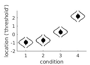
Figure 1. Each panel shows data from one observer testing under two experimental conditions with fits.
By visual inspection of Figure 1, it certainly seems like the location parameter is affected by the manipulation between the two conditions: For all 5 observers the PF for the 'red' condition
is shifted to the right relative to the 'blue' condition, although for some observers the effect is stronger compared to other observers. But when we analyze this with a Hierarchical Bayesian
model (using PAL_PFHB_fitModel), then ask for the violin plots for the mean location parameters in the two conditions:
>> pfhb = PAL_PFHB_fitModel(data,'gammaEQlambda',true,'prior','l','beta',[0.03 100]);>> PAL_PFHB_drawViolins(pfhb,'amu'); %amu is hyperparameter for location ('threshold') parameter
we get this:
Figure 2. Hyperparameters corresponding to the mean location hyperparameter for both conditions in the experiment
From this, it seems there is very little evidence that the location parameters differ between the conditions! This is not what we were expecting based on our visual inspection of the fitted PFs.
What is happening here is not that the analysis or the violin plot is incorrect, rather the results simply do not correspond to exactly what we are interested in. The violin plot shows the
posteriors for the location hyperparameters in the two conditions. Note however, that when we tried to gauge the experimental effect by visual inspection of Figure 1, we did this not by
estimating the mean location parameter across observers in the 'red' condition and the mean location parameter in the 'blue' condition and comparing those means. Instead we noted that
for each observer individually the red condition was shifted to the right relative to the blue condition. In other words: In our head, we estimated an effect of the manipulation for each observer
individually, then averaged those. In yet other words: When judging the effect, we completely disregarded the fact that the location parameters differed quite a bit between observers. This was
pretty smart of us, because that variance is not relevant to the question of whether location parameters are affected by condition. The problem with the estimates in Figure 2 is that these do not
disregard the differences between average location parameters between observers. This results in the large uncertainty (i.e., wide posteriors) on the estimates.
To give a simple (but unrealistic) analogy, imagine somebody invents a 'smart pill' that is supposed to increase the IQ of whoever takes it. In order to test whether it works, the inventor of the
smart pill finds five willing participants, measures their IQ both before and after taking the smart pill. The results are below:
Table 1.
It seems there is quite a bit of evidence that the smart pill works: All of the participants tested higher after the smart pill compared to before. Yet when we compare the difference between
the 'Before' and 'After' means relative to their standard errors we are hardly impressed. The problem is that the SEs for the 'Before' and 'After' means include the differences that participants
brought to the experiment that have nothing to do with how well the smart pill works. Some participants were much smarter than others. This example is similar to the scenario above
because here too we are not interested in how smart these participants were before or how smart they were after. Instead we are interested in whether they got smarter. So we do what
we were taught to do in our introductory statistics course: We reparameterize the model. You might think: I have taken an introductory statistics course but they never taught me to
reparameterize anything, they taught me to do a dependent-samples t-test here! Potato-Potahto. In a dependent-samples t-test the first thing to do is to calculate difference scores, either
'After' - 'Before' or vice versa.
If we do that, the data become:
Table 2.
Note that besides calculating the difference scores, we also calculated the average IQ for each participant (i.e., (Before + After)/2) even though these averages are not at all used in a
dependent-samples t-test as they do not tell us anything about how much difference the smart pill makes. We have reparameterized the model. No information was lost when
we did this. From these raparameterized data, we can still figure out what the IQ score of each participant was before and after the smart pill. We will not analyze the 'raw' IQs of participants
or the means of these IQs. Instead we will analyze the reparameterized data, specifically the difference scores. We see that the mean of these improvement scores is 8 points and the
standard error on that number is 2.53. So this would lend much more credibility to the idea that the pill increases IQ.
We need to have Palamedes do the same: Estimate for each observer individually what the effect was of the condition on the PF's location parameter and also estimate the mean of those
effects across participants, complete with posterior and credible intervals and all that. Or means and SEs and p-values if going the frequentist route. Reparameterization works for either.
That means we need to reparameterize the model: Instead of estimating location parameters for condition 1 and location parameters for condition 2, we will estimate, for each observer, the
average location across the two conditions but, of greater theoretical interest, also the difference in locations between the conditions.
We can instruct Palamedes to do this using a model matrix. Model matrices specify new reparameterized parameters (for the sake of convenience, henceforth reparameters) as
linear combinations of the raw parameters. If we symbolize the location parameters in condition 1 and condition 2 as a1 and a2 respectively, the average
location parameter, of course, is:
and the diference between location parameters is:
The model matrix that accomplishes the reparameterization simply contains the coefficients of these equations:
The model matrix has as many columns as there are conditions in the experiment. It has one row for each reparameter we want to estimate. Each row contains the coefficients to use in
the equations specifying the reparameter. Let us analyze these data again, but now estimating the reparameters defined by M instead of the raw location parameters:
>> pfhb = PAL_PFHB_fitModel(data,'gammaEQlambda',true,'prior','l','beta',[0.03 100],'a',M);>> PAL_PFHB_drawViolins(pfhb,'amu');
which gives:
Figure 3. Hyperparameters corresponding to the mean location hyperreparameters
Note that the x-axis now is labeled 'effect' and not 'condition' (as was the case in Figure 2). This is because the parameters represented in the figure no longer correspond to the location
parameters for each condition, but instead correspond to the reparameters: the mean and the difference, respectively, of the location parameters.
A few things to note from the violin plot: the mean parameter ('effect 1') has much more uncertainty associated with it compared to the difference parameter ('effect 2'). This is because the
observers differed quite a bit with respect to the average location of the PFs (see Figure 1). Much more so than they did with respect to the difference between the two PF locations.
Of theoretical interest, it is now clear that a value of zero is not very credible for the mean of the difference parameter (effect 2). This corresponds with our idea about the effect of
condition based on our casual inspection of Figure 1.
Note that even though we are not really interested in the average location of the PFs (i.e., a1*), leaving it out of the Model Matrix means that Palamedes would leave this 'effect' out of the model,
which effectively means that the model would be forced to keep the average location parameters (a1*) at 0, which would make for a very poor model. Note that we have reparameterized two
parameters (one location parameter for each of the two conditions) into two new reparameters (the average and difference between the two location parameters). Importantly,
these reparameterizations defined in the model matrix are orthogonal. In plain English, this means that each reparameter affects things that the other parameter has no control
over whatsoever. The value of a1* affects the average location parameter across conditions but does not affect the difference between the location
parameters whatsoever. Conversely, the value of a2* affects the difference between location parameters across conditions but does not affect the
average location parameters whatsoever. Whenever you reparameterize n parameters into n new parameters that are all mutually orthogonal, the reparameterized model is not constrained
in any way relative to the original model1. It is easy to verify whether two reparameters are orthogonal using the model matrix: Multiply the coefficients across the two rows,
then sum these products. If the sum equals 0, the parameters are orthogonal. Visually:
Figure 4. Verifying orthogonality of reparameterizations
The sum of the products indeed equals zero, confirming that the two reparameterizations are orthogonal. Having verified the two conditions above (we have as many reparameters as we had
'raw' parameters and the reparameterizations are orthogonal), we can rest assured that our reparameterization does not restrict our new model relative to its original parameterization.
Note that it can be useful to restrict a model. Remember that more parameters does not necessarily make for a better model. It can be useful to restrict (or constrain) the model that
Palamedes can fit by leaving effects out of the Model Matrix. As a matter of fact, the fit performed above used the Model Matrix [0.5 0.5] for the lapse rate parameter. In other words,
the model estimated only the average lapse rate between the two conditions and thereby did not allow for a difference between conditions. Effectively, this means that the model assumes
that the actual generating lapse rate was equal across conditions (but could still differ between observers). This would, generally speaking, be a sensible assumption that makes for a better
model (see Prins, 2024).
Leaving effects out of the model also allows a comparison between two versions of a model: One which includes the effect and one which does not. One could then compare the fit of the
two models using, for example, one of the information criteria (AIC, BIC, etc.). In the above example, one could compare the fit of a model that includes both
a1* and a2* (the difference parameter)
to one that includes only a1*. The former would allow the location parameters to differ, the latter would not.
It is perfectly fine to use different parameterizations for the different parameters of the PF. Above, we reparameterized the location parameter into the average location and the difference
between locations. We used a different reparameterization for the lapse rate in order to constrain the lapse rates to be equal between conditions. Finally, we did not reparameterize the slope parameters at all.
Designing Model Matrices: Tips and Tricks
Remember that any reparameterization that has as many reparameters as there are raw parameters and for which these reparameterizations are all mutually orthogonal does
not constrain your model. Designing a model matrix that targets specific research hypotheses while not constraining the model can be a bit of an art.
We'll go through some special matrices and some examples to demonstrate some general strategies and tricks.
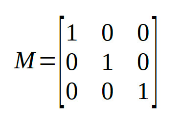
Identity Matrix
The identity matrix has 1s on the diagonal and zeros everywhere else. For three conditions:
The reparameters are identical to the raw parameters, i.e., the identity matrix doesn't really
reparameterize your model at all. In Palamedes fitting routines, the identity matrix is the default for the location and slope parameters of a PF.
Helmert Contrasts
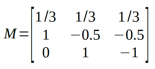
Use the first row of the matrix to define a reparameter that corresponds to the average. E.g., for three conditions: 1/3 1/3 1/3 as above. The
remaining rows can be so-called Helmert contrasts. The first Helmert contrast compares the first group against the groups in the higher conditions. With three conditions it would compare
the first condition to the average of the other two conditions. Thus, the new parameter will be:
So the corresponding row in the Model Matrix will be:
[1 -0.5 -0.5]
Note that the coefficients in the row add to zero. This is a good thing. If the coefficients add to zero, the row will be orthogonal to the first row (which defined the average). If the coefficients
do not add to zero, the row will not be orthogonal to the first row.
The second Helmert contrast compares the two conditions that were grouped together in the first Helmert contrast (i.e., conditions 2 and 3) against each other:
[0 1 -1]
Thus, the full model matrix is:
We leave it to the reader to verify that all pairs of rows in the matrix are mutually orthogonal.
The Palamedes routine PAL_Contrasts can generate a model matrix containing Helmert contrasts:
>>M = PAL_Contrasts(3,'Helmert') %type help PAL_Contrasts for details on usewhich gives: M =
1 1 1
2 -1 -1
0 1 -1 Note that each row is actually a multiple of the matrix given above such that all entries are whole numbers. Each row is simply a multiple of the corresponding row in the matrix above. This changes the interpretation of the parameter estimates. For example, in the matrix generated by PAL_Contrasts, the first reparameter corresponds to the sum (rather than the average) across the conditions. In general, we recommend creating model matrices for which the reparameters can be thought of to correspond to averages or differences between averages (e.g., the reparameter defined by the second row corresponds to [1 -0.5 -0.5], that is: 'condition 1 - the average of conditions 2 and 3'). In order to do this, for each row simply divide the coefficients by the sum of the positive coefficients in the row. Multiplying/dividing all coefficients in a row by a constant does not change whether the reparameterization defined by that row is or is not orthogonal with the other reparameterizations in the matrix. Note that the order of conditions is arbitrary, so you can the shuffle the order of the columns around if that makes for more theoretically meaningful comparisons (but the entire column must be shifted, not just columns within individual rows), resulting for example in:
Polynomial Contrasts
Polynomial contrasts can be used to perform a so-called trend analysis and can be particularly useful if the independent variable defining the various conditions is measured on an interval
scale of measurement (adaptation duration, for example). When a model matrix that utilizes polynomial contrasts is used to reparameterize parameters and all but the first m
reparameters are zero, the modeled parameters will fall along a polynomial curve of order m - 1. For example, let's say you perform an experiment and use four different adaptation
durations of an adapting stimulus: 0, 10, 20, and 30 seconds. The data with fitted psychometric functions looks like this (note that slopes were assumed to be equal between conditions for
this fit):
The violin plots for the raw location parameters look like this:
It seems clear that the location parameter values generally increase with adaptation duration (that would be the 'linear trend'), but it is less clear whether the bend in the relationship is 'real'
or not (that would be the 'quadratic trend'). A model matrix containing polynomial contrast addresses this question. The function PAL_Contrast can generate a model matrix for a trend
analysis:
>>M = PAL_Contrasts(4,'polynomial') %type help PAL_Contrasts for details on usewhich gives: M =
1 1 1 1
-3 -1 1 3
1 -1 -1 1
-1 3 -3 1 These four reparameters are orthogonal. Using this matrix to reparameterize the location parameters, then asking for the violin plots give this:
'effect 1' is the reparameter defined by the first row of M, in other words the sum of the four location parameters. The 'effect 2' reparameter is the linear trend. We see that, as expected, it
is likely to have a high, positive value (and that a value of 0 is effectively impossible). This confirms that thresholds indeed tend to rise with adaptation duration. The 'effect 3'
reparameter is the quadratic trend and, simply put, allows the line to have a bend. In this violin plot, the posterior for the quadratic trend is a bit smooshed, but we can create a violin plot for 'effect 3' separately using:
>>PAL_PFHB_drawViolins(pfhb,'effect',3)It is now clear that a value of 0 is not very likely for the quadratic trend which may suggest that the bend is 'real'.
Tree Diagram Method
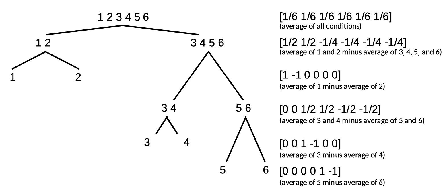
Orthogonal contrasts may also be constructed by using a tree diagram, in which the k conditions are first divided into two groups by one reparameter, and each of the two
resulting groups is then further divided into two groups by additional reparameters. This process continues until no further divisions are possible. For example, if we start with
k = 6 conditions, we could use the following tree diagram to construct a set of 6 orthogonal reparameterizations:
The full matrix then is:
We leave it up to the reader to verify that these 6 reparameterizations are indeed all mutually orthogonal.
Note that Helmert contrasts can be formed using a tree diagram. Note also that while any set of contrasts that divides parameters according to a tree diagram will result in a set of
orthogonal contrasts, a set of contrasts may still be orthogonal even in cases where they do not follow a tree diagram. One example of this is the set of polynomial contrasts given above.
Some more examples are discussed below.
Factorial Designs
2 × 2 Factorial design
Let's say you want to investigate the effect of two independent variables (IV A and IV B) on the location parameter of the PF. Each IV has two levels and these are fully crossed resulting
in four conditions. It is natural to define reparameters to correspond to the main effects and the interaction between the IVs. There are 4 raw parameters, thus we want to define
4 reparameters that are orthogonal. How to go about finding the appropriate model matrix? Refer to the table below as we go through this.
The first reparameter is easy:
As in all examples so far, it corresponds to the average across all conditions. However, for now, we will use only integers for coefficients and we will normalize the coefficients later. Thus
our first row, for now, will be:
[1 1 1 1]
Let's make our second reparameter correspond to the main effect of IV A. Also easy. The reparameter will be the average of conditions under level 1 of A minus the
average of conditions under level 2 of A (but, again for now we will use integers only):
[1 1 -1 -1]
Our third reparameter will correspond to the main effect of IV B. Just as easy as the previous one. The reparameter will be the average of conditions under level 1 of B
minus the average of conditions under level 2 of B (but, again for now we will use integers only):
[1 -1 1 -1]
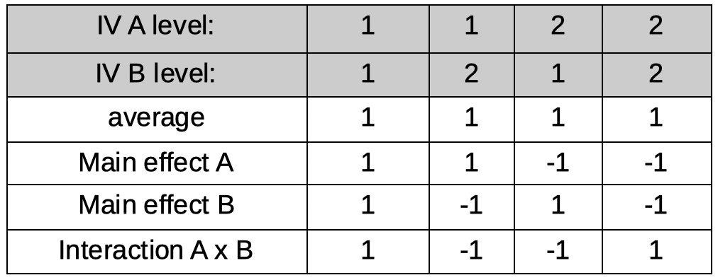
Our last parameter will correspond to the A × B interaction. Conceptually not as easy as the first three reparameters, but lucky for us, in practice very easy to create. Interaction
reparameters can simply be found by multiplying the coefficients across the main effect reparameterizations (there is a reason interactions are often notated using the
multiplication symbol [e.g., 'A × B'], as we did above!). Thus, our last reparameter is defined by:
[1×1 1×-1 -1×1 -1×-1]
or:
[1 -1 -1 1]
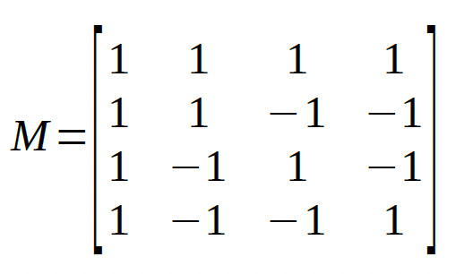
The full matrix:
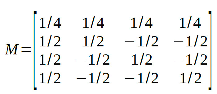
The four reparameters are all mutually orthogonal. As a last step, let's normalize the matrix such that the reparameters can be interpreted as averages or differences
between averages (this will not change whether rows are orthogonal):
At first glance, the interaction contrast might not make much sense. Let's take a look at the non-normalized coefficients:
[1 -1 -1 1]
Thus the interaction reparameter is defined as:
A1B1 - A1B2 - A2B1 + A2B2
(where e.g., A1B2 refers to the condition that is under level 1 of Factor A and level 2 of Factor B)
In order to see that this indeed corresponds to the interaction of the two Factors note that this is equivalent to
(A2B2-A2B1)-(A1B2-A1B1)
The term within the first set of parentheses (i.e., A2B2 - A2B1) is the effect that IV B has within the second level of IV A. The term within the second set of parentheses (i.e., A1B2 - A1B1)
is the effect IV B has within the first level of IV A. Thus, when the effect of B is the same in both levels of A
(i.e., Factor A and Factor B do not interact), the interaction reparameter equals 0. If the effect of B differs
between the two levels of A (i.e., Factor A and Factor B interact), the reparameter will take on a value other than 0.
Note that this model matrix could not have been created using the tree method above, but nevertheless consists of reparameterizations that are all mutually orthogonal.
2 × 3 Factorial design
Let's say one of your IVs (A) in a factorial design has 2 levels and the other (B) has 3 levels, resulting in 6 conditions (see Table below for a listing of the conditions).
Let's see if we can find 6 orthogonal reparameters that correspond to the average, the main effects and the interactions. The first reparameter is the average (but
again for now let's stick to integers and actually make it the sum):
[1 1 1 1 1 1]
Next, the main effect of A. It might help here to consider how many degrees of freedom are associated with the main effect for A. From our introductory statistics class we remember
(hopefully) that a factor with two levels has one degree of freedom associated with it. That translates here to needing only 1 reparameter to represent the differences among
the two levels of the factor. The reparameter corresponds to the average across, say, the conditions in the first level of A minus the average across the conditions in the second
level of A. Using the ordering of the 6 conditions shown in the table above, and again sticking to integers for now, the coefficients for the reparameter are:
[1 1 1 -1 -1 -1]
Now for the main effects of factor B. No, the plural 's' in 'effects' is not a typo. Remember that a main effect for an IV with three levels has 2 degrees of freedom, which translates here
as requiring two reparameters to define the main effects for Factor B. It is easier to forget for now about the other Factor and pretend we're designing reparameters
for a simple one-factor experiment where the factor has three levels: B1, B2, and B3. Let's use Helmert contrasts here just like we did way above when we were considering a simple,
one-factor experiment with three levels and used Helmert contrasts. However, we'll stick again to using only integers for now and use:
[2 -1 -1]
and
[0 1 -1]
expanding this across all six conditions in our experiment gives the reparameters labeled 'main effect B1' and 'main effect B2' in the table above. Note that we simply made
two copies of the coefficients: One for the conditions under level 1 of A, the other for conditions under level 2 of A.
All that is left is to find the two reparameters that will define the interactions (plural 's' intended!). Note that again, the number of reparameters needed is equal to
the degrees of freedom associated with the effect. In a 2 × 3 the number of degrees of freedom associated with the interaction equals 2. Practically, the coefficients for these are easy
to find. One interaction will be the interaction between the main effect of A and the first main effect on B (labeled B1 above). The coefficients correspond again simply to the products of the two interacting
main effects, so we simply multiply the coefficients in the 'main effect A' row with the coefficients in the 'main effect B1' row. In a similar fashion, we can find the coefficients for the
A × B2 interaction. You may have realized by now that we chose to stick to integer values for coefficients for now because that makes the multiplication of coefficients to find the
interactions much easier. Normalization of the coefficients in the table results in the final model matrix:
As usual, we will leave it up to the reader to verify that all 6 reparameterizations are orthogonal.
Combining Methods Example: Tree method and Factorial design
The different methods above can be combined. To illustrate this, let's consider an experiment that investigates the effects of the contrast (Factor A) and the duration (Factor B) of an
adapting stimulus on the detectability of a consequent stimulus. Of interest is how these factors affect the location parameter of the PF describing proportion correct in the detection
task. Three levels of duration (0, 100, and 1000 msec) and two levels of contrast are used (10 and 20 cdm-2). This appears to be a simple 2 × 3 Factorial design with
6 conditions (for which we derived a possible model matrix above) until we realize that when duration equals 0 msec, the variable contrast is meaningless. There really are only 5
conditions (listed in the Table below) that are perhaps most easily thought of as a 2 (duration = 100 and 1000 msec) × 2 (contrast = 10 and 20 cdm-2) factorial design with an added control
condition (in which there is no adapting stimulus).
Many different model matrices can be created to reparameterize these 5 conditions into 5 orthogonal reparameters. However, we should create one that isolates interesting
research questions. Let's say we have a specific interest in determining whether duration and contrast interact (when there is in fact an adapting stimulus). So we want one of the 5
reparameters to correspond to that interaction. What we can do to accomplish this is to first use the tree method above to identify a reparameter that separates the 5
conditions into the control condition on the one hand and the 2 × 2 section of the design on the other, then to use the reparameterization for the 2 × 2 design derived above to
reparameterize the 2 × 2 section of the design. The coefficients in the table below do just that.
Normalization of the coefficients leads to:
Another Combining Methods Example: Factorial design with polynomial contrasts
Let's say you have a 2 × 4 design where the 4 levels of Factor B differ on some quantitative variable. For example, let's say the four conditions in the example above under 'polynomial contrasts'
were tested again but were now actually measured twice: once monocularly and once binocularly. That makes it a 2 × 4 Factorial design. Let's say the violin plots for the raw (i.e., not reparameterized) location
parameters look like this:
Conditions 1-4 are the monocular conditions, conditions 5-8 are the binocular conditions. It seems clear that there is a linear trend main effect: in both the monocular and binocular
viewing conditions, the location parameters generally increase with adaptation duration. However, it seems that they increase a bit faster in the binocular viewing condition compared
to the monocular conditions. This would be the linear trend on adaptation duration × viewing condition interaction. Let's set up the model matrix. We have 8 raw location parameters, we
would like 8 orthogonal reparameters. This may seem like a difficult task, but it is not. The first one is routine by now. It is the average location:
M(1,:) = [1/8 1/8 1/8 1/8 1/8 1/8 1/8 1/8];
Next, let's work on the main effect of Factor A (monocular versus binocular viewing condition). There are two levels, thus one degree of freedom or one reparameter. Also easy: we'll make it
the sum of the location parameters under binocular viewing minus the sum of the location parameters under the monocular viewing conditions. This is essentially the same 'difference'
reparameter from the very first example above except now it has to be expanded because it is crossed with the second variable. If the order in which the conditions are numbered in the data
structure is A1B1 A1B2 A1B3 A1B4 A2B1 A2B2 A2B3 A2B4 (i.e., conditions are ordered as in the violin plot above) then our second reparameter is:
M(2,:) = [-1 -1 -1 -1 1 1 1 1];
The natural next thing to work on is the main effects of Factor B. Yes, that's again a plural 'effects' because Factor B has 4 levels, 3 degrees of freedoms and thus 3 reparameters that
define the main effects of this Factor. Just like above in the example where adaptation duration was the only factor, we will use polynomial contrasts. But, because of the other Factor, we will need to expand again
to cover both instances of each adaptation duration:
M(3,:) = [-3 -1 1 3 -3 -1 1 3];
M(4,:) = [1 -1 -1 1 1 -1 -1 1];
M(5,:) = [-1 3 -3 1 -1 3 -3 1];
These are the main (as in 'main effect') linear trend on adaptation duration, the main quadratic trend on adaptation duration, and the main cubic trend on adaptation duration, respectively. We have
5 reparameters so far, so we need three more to complete the set. Of course, these will be the interaction effects. Remember that in a 2×4 design there are three degrees of freedom associated with the
interaction and thus three reparameters. We can find these again simply by multiplying contrasts coefficients across the main effects:
M(6,:) = M(2,:).*M(3,);
M(7,:) = M(2,:).*M(4,);
M(8,:) = M(2,:).*M(5,);
These are the viewing condition × linear trend on adaptation duration interaction ('does the general rate of increase of the location parameter differ between monocular and binocular viewing?'),
viewing condition × quadratic trend on adaptation duration interaction ('does the quadratic trend differ between monocular and binocular viewing?'), and the viewing condition × cubic trend on
adaptation duration interaction ('does the cubic trend differ between monocular and binocular viewing), respectively.
That's it. These 8 reparameterizations are all mutually orthogonal (but feel free to check). Analyzing the data again with the reparametrized location parameters gives these violin plots:
From the violin plot we see that reparameter 3 (main linear trend on adaptation duration) is positive and very unlikely to include 0 confirming that, averaged between monocular and
binocular viewing conditions, the location parameters increase with adaptation duration. We also see that reparameter 6 (viewing condition × linear trend on adaptation duration) is
positive and unlikely to include 0 suggesting that the apparent faster rate of increase of location parameter with adaptation duration when stimuli are viewed binocularly compared to monocularly is 'real'.
Constraining Parameters
You can constrain a parameter to have equal values across all conditions by including only a single row in the model matrix that defines a reparameter as the average of the
parameter value across the conditions. For example, if there are three conditions:
M = [1/3 1/3 1/3];
This is the default for the lapse parameter. Using this model matrix will constrain the lapse rate to be equal across the conditions, essentially implementing the assumption that the true,
generating value of the parameter is equal in all conditions. This is generally a reasonable assumption and allows you to reduce model complexity by reducing the number of free parameters.
This is a good thing! Including unnecessary parameters such as an individual lapse rate for each condition makes for a poor model. Reducing model complexity by constraining parameters
will also generally increase the likelihood that your fit will converge.
Note that it may not always be reasonable to assume that the lapse rate is equal across all conditions. For example, one of the experimental manipulations in Prins, Behavior
Research Methods, 2024 manipulated the attentional load of a secondary task. Such a manipulation is likely to affect the lapse rate on the primary task. In such a situation, it makes
sense to allow lapse rates to differ between conditions under different levels of attentional load while constraining lapse rates to be equal within the different levels of attentional load. Prins used
a 3×2×2×2 Factorial design where the Factor with three levels manipulated the attentional load. Thus, the first 8 conditions had a low attentional load, the next 8 had a medium attentional load,
while the remaining 8 conditions had a high attentional load. The matrix that is used to constrain lapse rates within, but not between, attentional load conditions is
You can also constrain model parameters by leaving out any combination of the reparameters from a model matrix. To give one example, in the analysis under 'Polynomial Contrasts' above
we reparameterized the four location parameters into four orthogonal reparameters using polynomial contrasts. Thus, this reparameterization did not constrain the location parameters at all.
We can constrain the location parameters to increase strictly linearly as a function of adaptation duration by including only the first and second rows of the
model matrix (i.e., the 'intercept' and linear trend). thus the model matrix we'll use is:
M = [ 1 1 1 1;
-3 -1 1 3] The fitted psychometric functions looks like this:
Note that now the location parameters are indeed equally spaced and thus would all fall on a first-order polynomial (i.e., a straight line). Casual inspection of this graph confirms once again that the bend (i.e.,
quadratic trend) in the original fit was real: Here we left it out and the result is that the constrained psychometric functions do not appear to describe the data very well. Formal procedures exist
to compare the constrained model against the unconstrained model (e.g., Bayes Factors, one of the information criteria, or the likelihood ratio test).
Prins, N. (2024). Easy, bias-free Bayesian hierarchical modeling of the psychometric function using the Palamedes Toolbox. Behavior Research Methods, 56(1), 485-499. https://doi.org/10.3758/s13428-023-02061-0