Oh, that pesky lapse rate.
What is going on in the figure below? The supposed 'best-fitting' function (shown in black) doesn't seem to model the observed proportions correct very well, while
the high-density region does seem to be on target.
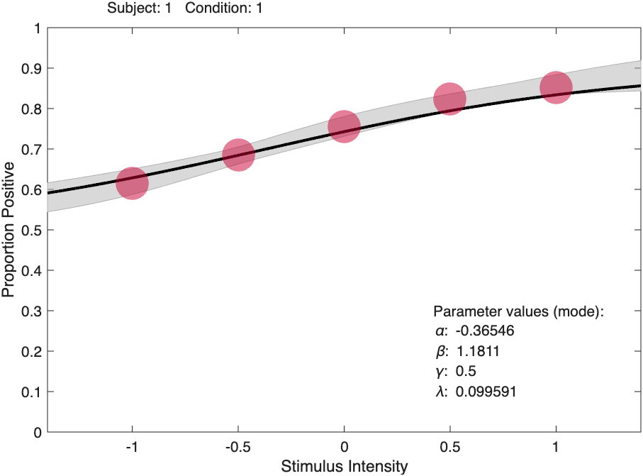 Figure 1. Created using code:
data.x = [-1 -.5 0 .5 1];
data.n = [600 600 600 600 600];
data.y = PAL_PF_SimulateObserverParametric([0 1 .5 0],data.x,data.n,@PAL_Logistic);
pfhb = PAL_PFHB_fitModel(data,'nsamples',100000);
PAL_PFHB_inspectFit(pfhb);
(data.y for this figure was: [369 411 453 494 511])
Long story short, the discrepancy happens because the lapse rate was allowed to vary but no attempt was made to collect information on the value of the lapse rate and, surprise, the data contain virtually no information on the lapse rate. As a result there is a high redundancy among your free parameters (here: the location ['threshold'], slope and lapse rate parameters). Consider a graph like that above to be a diagnostic of this serious problem with your data. To learn more about what went wrong and to find out how to prevent this issue from occurring in the first place and how to manage it once it has occurred, read on.
The long story goes like this:
The discrepancy occurs because the black curve is derived under the assumption that the free parameters are not correlated while the 68% high-density region does not make that assumption. In sensibly collected data, correlation among parameter values is kept at bay. The data above were not sensibly collected. As a result, this assumption is violated quite severely in the data above. Yep, because the lapse rate was 'allowed to vary' but the data contain virtually no information about the lapse rate. Generally speaking, this problem will arise whenever there were no, or very few, trials were collected at stimulus intensities where the true, generating psychometric function has reached near asymptotic levels (Prins, 2012) Unfortunately, it is very common for researchers to allow the lapse rate to vary without having collected data at near-asymptotic data. One such scenario is when the original psi-method is utilized to place stimuli but the data are then fitted with a free lapse rate (Prins, 2013).
By default, PAL_PFHB_inspectFit uses the mode of the posterior distribution as the criterion for 'best-fitting' function (this can be overridden, type 'help PAL_PFHB_inspectFit'). However, estimating the mode of a posterior defined across three parameters is difficult and computationally intensive. So, what is typically done (and what Palamedes does also) is to take a shortcut. The shortcut is to find the mode in each parameter's marginal posterior distribution and assume that the mode in the 3D posterior is located at the intersection of the three marginal modes. However, that works only insofar as the parameters are independent. A simple 2D example can demonstrate this. In Figure 2 below there are nine objects that vary in two dimensions: color and shape. The modal object is 'green circle': There are more green circles than any other object. That was easy.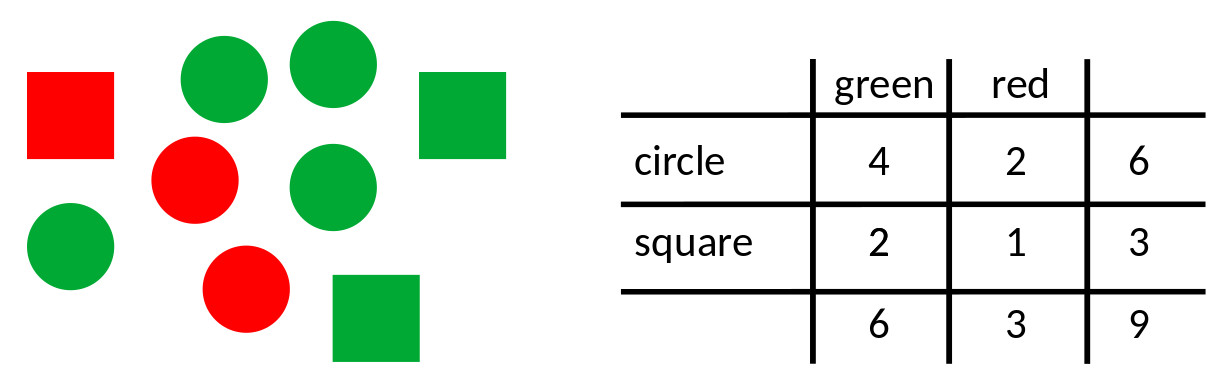 Figure 2.
The shortcut we use when things are not so easy is to find the modes in the marginal distributions (i.e., what is the most common color and what is the most common shape) and to assume that the modal object has the combination of most common color and the most common shape. For the example in Figure 2 this works: The modal color is 'green' (6 objects are green, 3 objects are red) and the modal shape is 'circle' (there are 6 circles and 3 squares). And low and behold, the most common object is 'green circle'. This worked here because color and shape are independent (e.g., if an object is red, there is a 2/3 chance that it is a circle and 1/3 chance that it is a square and the same is true if the object is green). Now consider the objects in Figure 3. The modal color is again 'green', the modal shape is again 'circle'. However, here the modal object is not 'green circle'. The shortcut failed here because color and shape are correlated, (e.g., if an object is red, it is certain to be a circle, but if an object is green it is likely to be a square).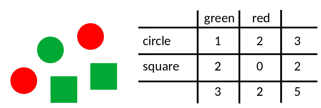 Figure 3.
Now back to our psychometric function. The parameter values of the black curve (as listed in the figure) correspond to the marginal modes of location, slope, and lapse rate. That is, -0.36546 is the most likely value for the location parameter, 1.1811 is the most likely value for the slope and 0.099591 is the most likely value for the lapse rate. However, the particular combination of those parameter values is not very likely (revisit the circles and squares example if that doesn't make sense). The discrepancy is due to the high correlations between the parameters in this example. Figure 4 shows the scatterplot between location values and lapse rate values sampled from the posterior distribution [as visualized by PAL_PFHB_inspectParam(pfhb,'a','l')] and Figure 5 shows the scatterplot between slope values and lapse rate values.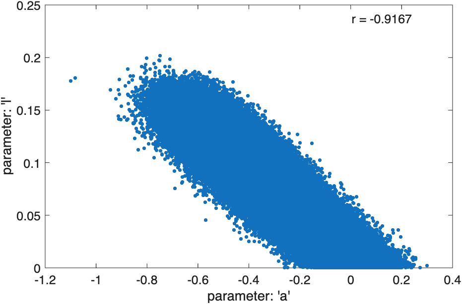 Figure 4.
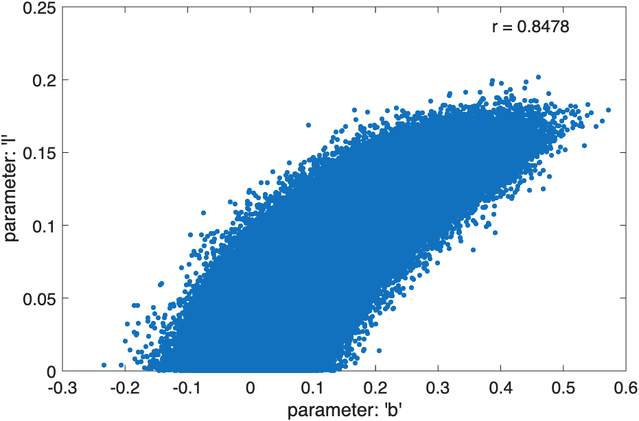 Figure 5.
To create this page, we did go through the time-consuming and computationally intensive process of estimating the full 3D posterior and its mode without relying on the assumption that parameters are independent. Figure 6 shows the 68% high-density region for the posterior. The mode in this full posterior is shown as the red dot and corresponds to the parameter value combination: location = -0.292, slope = 1.272, lapse rate = 0.066. This curve is shown in the top panel Figure 7 in red. It does a much better job of fitting the observed proportions correct compared to the curve based on the marginal modes (again shown in this figure in black). All is well and good with this fit. Except not really....
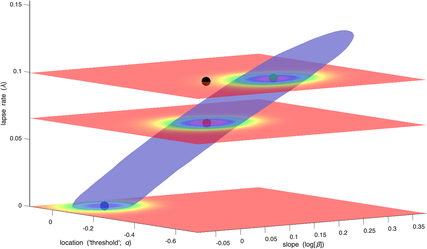 Figure 6. The solid corresponds to the 68% high-density region of the 3D posterior distribution. The black dot is located at the intersection of the marginal modes of the location, log(slope),
and lapse rate parameters). The red dot is located at the mode of the 3D posterior distribution. The blue dot is located at the mode of the 'slice' through the posterior at lapse rate = 0. The green
dot is located at the mode of the 'slice' through the posterior at lapse rate = 0.1.
Figure 6. The solid corresponds to the 68% high-density region of the 3D posterior distribution. The black dot is located at the intersection of the marginal modes of the location, log(slope),
and lapse rate parameters). The red dot is located at the mode of the 3D posterior distribution. The blue dot is located at the mode of the 'slice' through the posterior at lapse rate = 0. The green
dot is located at the mode of the 'slice' through the posterior at lapse rate = 0.1.
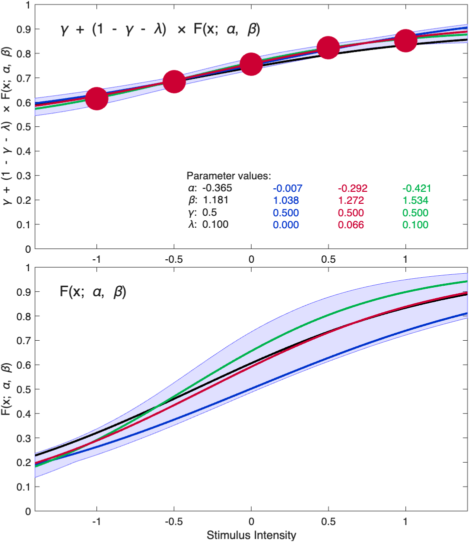 Figure 7. Psychometric Functions located at the colored dots in Figure 6. See text for details.
What Figures 6 and 7 demonstrate is that, because of the high degree of correlation (or 'redundancy') among the parameters, the true mode in the 3D posterior is actually just one function in a family of functions that all fit the data about equally well. Figures 6 and 7 shows three functions in this family in red, green, and blue where the colors of the curves correspond to the colors of the dots in Figure 6. Note that, within the stimulus range, the three functions are virtually identical. It is only outside the stimulus range (especially at intensities above the highest intensity that was used) where the functions diverge.
While it appears from Figures 1 and 7, top panel, that the location parameter (as well as the other parameters) are estimated quite precisely (i.e., the high-density region is quite narrow), this is actually not the case. What the figure shows is that the stimulus intensity at which the function reaches, say, 75% correct is estimated quite precisely. The problem is that this stimulus intensity depends not only on the location parameter but also on the other parameters of the PF, here the slope and the lapse rate. A simple analogy might help to make the point: let's say the number of animals at the local animal shelter is precisely estimated to equal 100. However, having a precise estimate of the total number of animals at the shelter does not mean you have a precise estimate of the number of dogs that are the shelter. This is because a whole family of models all correspond to the total number of animals being 100 (e.g., 25 dogs and 75 cats, 75 dogs and 25 cats, etc., etc.). To show that the estimate of the location parameter is not very precise at all, Figure 7, bottom panel, display the functions that depend only on the 'perceptual' part of the psychometric function (i.e., the part we would typically be interested in: F(x; α, β) in the standard equation for the psychometric function shown below), leaving out the 'decision' part of the function, ruled by the 'nuisance' parameters guess and lapse rate and include its 68% high-density region in the figure. It is obvious that even though the full psychometric function is estimated quite precisely, the 'perceptual part' is not estimated very precisely at all (think of the former as the number of pets at the shelter and the latter as the number of dogs at the shelter).
Note that the problem is quite severe even though the fit is based on a very high (some would say excessive) number of trials (3,000). The problem continues to exist even with 3,000 trials because the 3,000 trials were not wisely spent. The 3,000 trials were all obtained at a set of stimulus intensities for which a family of PFs can produce similar probabilities correct despite varying quite a bit in their parameter values (the blue, green, and red curves in Figure 6 correspond to three members of that family). One way out of this is to obtain a more precise estimate for any one of the parameters, even the 'nuisance' lapse rate parameter (in the animal shelter analogy, one can improves one's estimate of the number of dogs by estimating the number of cats in addition to the total number of animals!). A good way to isolate one of the three parameters is to include a number of 'free trials' which are trials placed at a very high intensity so that it can be assumed that an incorrect response for these trials is almost certainly due to a lapse (see e.g., Swanson & Birch, 1992; Prins, 2012). Thus, some of these trials would have been more wisely spent on these 'free trials'. These would have the direct effect of narrowing the likely range for the lapse rate, reducing the redundancy among parameters, and reducing the uncertainty in the location and slope parameters. Note that the 3,000 trials in this example resulted in virtually no information gain regarding the value of the lapse rate. Figure 8 shows the estimated marginal posterior distribution for the lapse rate (figure created with PAL_PFHB_inspectParam). After 3,000 trials, the posterior is only mildly narrower compared to the prior distribution used for the lapse rate (beta with a = 1 and b = 10). Essentially, after 3,000 trials we still have no idea what the value of the lapse rate might be and, because the lapse rate is highly redundant with the location and slope parameters, we don't have a very good idea what their value might be either.
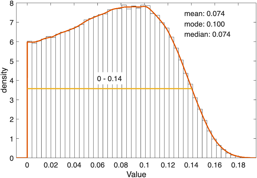 Figure 8.
You may wonder: How many trials should be free trials? The adaptive psi-marginal method (Prins, 2013) can be set up to inject free trials whenever this is the most efficient manner in which to increase information regarding the parameters of direct interest (e.g., location and/or slope parameters).
There are other strategies also that will reduce the problem. One is to combine multiple conditions into a single analysis and estimate a single, shared lapse rate across all conditions. This effectively implements the assumption that the lapse rate is independent of condition (i.e., a subject is just as likely to lapse in condition 1 as they are to lapse in condition 2 or any other condition). Usually this is a fair assumption as the lapse rate, by definition, is independent of the characteristics of the stimulus. By combining multiple conditions into a single analysis in this manner, the lapse rate estimate will be based on more trials and thus be more accurate and precise (Prins, Behavior Research Methods, 2023). Combining data from multiple observers into a single hierarchical analysis will also reduce the problem. Each observer's lapse rate estimate will be informed by the lapse rate estimates for the other observers through the hierarchical structure of the model (Prins, Behavior Research Methods, 2023). You can also combine multiple conditions of multiple observers into a single analysis. Sounds complicated? It's not, see PAL_PFHB_MultipleSubjectsAndConditions_Demo.m in the PalamedesDemos folder. Even with this strategy, it is still a good idea to place some observations at intensities conducive to avoiding parameter redundancy. Finally, you should always use a prior distribution for the lapse rate (and other parameters for that matter) that reflect your belief in what the values for these parameters may be. Different priors would be appropriate for animals, young children, experienced psychophysical observers, or undergraduate students satisfying credit requirements for an introductory psychology course. The less precise your prior, the bigger the problem discussed on this page becomes.
Figure 1. Created using code:data.x = [-1 -.5 0 .5 1];
data.n = [600 600 600 600 600];
data.y = PAL_PF_SimulateObserverParametric([0 1 .5 0],data.x,data.n,@PAL_Logistic);
pfhb = PAL_PFHB_fitModel(data,'nsamples',100000);
PAL_PFHB_inspectFit(pfhb);
(data.y for this figure was: [369 411 453 494 511])
Long story short, the discrepancy happens because the lapse rate was allowed to vary but no attempt was made to collect information on the value of the lapse rate and, surprise, the data contain virtually no information on the lapse rate. As a result there is a high redundancy among your free parameters (here: the location ['threshold'], slope and lapse rate parameters). Consider a graph like that above to be a diagnostic of this serious problem with your data. To learn more about what went wrong and to find out how to prevent this issue from occurring in the first place and how to manage it once it has occurred, read on.
The long story goes like this:
The discrepancy occurs because the black curve is derived under the assumption that the free parameters are not correlated while the 68% high-density region does not make that assumption. In sensibly collected data, correlation among parameter values is kept at bay. The data above were not sensibly collected. As a result, this assumption is violated quite severely in the data above. Yep, because the lapse rate was 'allowed to vary' but the data contain virtually no information about the lapse rate. Generally speaking, this problem will arise whenever there were no, or very few, trials were collected at stimulus intensities where the true, generating psychometric function has reached near asymptotic levels (Prins, 2012) Unfortunately, it is very common for researchers to allow the lapse rate to vary without having collected data at near-asymptotic data. One such scenario is when the original psi-method is utilized to place stimuli but the data are then fitted with a free lapse rate (Prins, 2013).
By default, PAL_PFHB_inspectFit uses the mode of the posterior distribution as the criterion for 'best-fitting' function (this can be overridden, type 'help PAL_PFHB_inspectFit'). However, estimating the mode of a posterior defined across three parameters is difficult and computationally intensive. So, what is typically done (and what Palamedes does also) is to take a shortcut. The shortcut is to find the mode in each parameter's marginal posterior distribution and assume that the mode in the 3D posterior is located at the intersection of the three marginal modes. However, that works only insofar as the parameters are independent. A simple 2D example can demonstrate this. In Figure 2 below there are nine objects that vary in two dimensions: color and shape. The modal object is 'green circle': There are more green circles than any other object. That was easy.
Figure 2.
The shortcut we use when things are not so easy is to find the modes in the marginal distributions (i.e., what is the most common color and what is the most common shape) and to assume that the modal object has the combination of most common color and the most common shape. For the example in Figure 2 this works: The modal color is 'green' (6 objects are green, 3 objects are red) and the modal shape is 'circle' (there are 6 circles and 3 squares). And low and behold, the most common object is 'green circle'. This worked here because color and shape are independent (e.g., if an object is red, there is a 2/3 chance that it is a circle and 1/3 chance that it is a square and the same is true if the object is green). Now consider the objects in Figure 3. The modal color is again 'green', the modal shape is again 'circle'. However, here the modal object is not 'green circle'. The shortcut failed here because color and shape are correlated, (e.g., if an object is red, it is certain to be a circle, but if an object is green it is likely to be a square).
Figure 3.
Now back to our psychometric function. The parameter values of the black curve (as listed in the figure) correspond to the marginal modes of location, slope, and lapse rate. That is, -0.36546 is the most likely value for the location parameter, 1.1811 is the most likely value for the slope and 0.099591 is the most likely value for the lapse rate. However, the particular combination of those parameter values is not very likely (revisit the circles and squares example if that doesn't make sense). The discrepancy is due to the high correlations between the parameters in this example. Figure 4 shows the scatterplot between location values and lapse rate values sampled from the posterior distribution [as visualized by PAL_PFHB_inspectParam(pfhb,'a','l')] and Figure 5 shows the scatterplot between slope values and lapse rate values.
Figure 4.
Figure 5.
To create this page, we did go through the time-consuming and computationally intensive process of estimating the full 3D posterior and its mode without relying on the assumption that parameters are independent. Figure 6 shows the 68% high-density region for the posterior. The mode in this full posterior is shown as the red dot and corresponds to the parameter value combination: location = -0.292, slope = 1.272, lapse rate = 0.066. This curve is shown in the top panel Figure 7 in red. It does a much better job of fitting the observed proportions correct compared to the curve based on the marginal modes (again shown in this figure in black). All is well and good with this fit. Except not really....
Figure 6. The solid corresponds to the 68% high-density region of the 3D posterior distribution. The black dot is located at the intersection of the marginal modes of the location, log(slope),
and lapse rate parameters). The red dot is located at the mode of the 3D posterior distribution. The blue dot is located at the mode of the 'slice' through the posterior at lapse rate = 0. The green
dot is located at the mode of the 'slice' through the posterior at lapse rate = 0.1.
Figure 7. Psychometric Functions located at the colored dots in Figure 6. See text for details.
What Figures 6 and 7 demonstrate is that, because of the high degree of correlation (or 'redundancy') among the parameters, the true mode in the 3D posterior is actually just one function in a family of functions that all fit the data about equally well. Figures 6 and 7 shows three functions in this family in red, green, and blue where the colors of the curves correspond to the colors of the dots in Figure 6. Note that, within the stimulus range, the three functions are virtually identical. It is only outside the stimulus range (especially at intensities above the highest intensity that was used) where the functions diverge.
While it appears from Figures 1 and 7, top panel, that the location parameter (as well as the other parameters) are estimated quite precisely (i.e., the high-density region is quite narrow), this is actually not the case. What the figure shows is that the stimulus intensity at which the function reaches, say, 75% correct is estimated quite precisely. The problem is that this stimulus intensity depends not only on the location parameter but also on the other parameters of the PF, here the slope and the lapse rate. A simple analogy might help to make the point: let's say the number of animals at the local animal shelter is precisely estimated to equal 100. However, having a precise estimate of the total number of animals at the shelter does not mean you have a precise estimate of the number of dogs that are the shelter. This is because a whole family of models all correspond to the total number of animals being 100 (e.g., 25 dogs and 75 cats, 75 dogs and 25 cats, etc., etc.). To show that the estimate of the location parameter is not very precise at all, Figure 7, bottom panel, display the functions that depend only on the 'perceptual' part of the psychometric function (i.e., the part we would typically be interested in: F(x; α, β) in the standard equation for the psychometric function shown below), leaving out the 'decision' part of the function, ruled by the 'nuisance' parameters guess and lapse rate and include its 68% high-density region in the figure. It is obvious that even though the full psychometric function is estimated quite precisely, the 'perceptual part' is not estimated very precisely at all (think of the former as the number of pets at the shelter and the latter as the number of dogs at the shelter).
Note that the problem is quite severe even though the fit is based on a very high (some would say excessive) number of trials (3,000). The problem continues to exist even with 3,000 trials because the 3,000 trials were not wisely spent. The 3,000 trials were all obtained at a set of stimulus intensities for which a family of PFs can produce similar probabilities correct despite varying quite a bit in their parameter values (the blue, green, and red curves in Figure 6 correspond to three members of that family). One way out of this is to obtain a more precise estimate for any one of the parameters, even the 'nuisance' lapse rate parameter (in the animal shelter analogy, one can improves one's estimate of the number of dogs by estimating the number of cats in addition to the total number of animals!). A good way to isolate one of the three parameters is to include a number of 'free trials' which are trials placed at a very high intensity so that it can be assumed that an incorrect response for these trials is almost certainly due to a lapse (see e.g., Swanson & Birch, 1992; Prins, 2012). Thus, some of these trials would have been more wisely spent on these 'free trials'. These would have the direct effect of narrowing the likely range for the lapse rate, reducing the redundancy among parameters, and reducing the uncertainty in the location and slope parameters. Note that the 3,000 trials in this example resulted in virtually no information gain regarding the value of the lapse rate. Figure 8 shows the estimated marginal posterior distribution for the lapse rate (figure created with PAL_PFHB_inspectParam). After 3,000 trials, the posterior is only mildly narrower compared to the prior distribution used for the lapse rate (beta with a = 1 and b = 10). Essentially, after 3,000 trials we still have no idea what the value of the lapse rate might be and, because the lapse rate is highly redundant with the location and slope parameters, we don't have a very good idea what their value might be either.
Figure 8.
You may wonder: How many trials should be free trials? The adaptive psi-marginal method (Prins, 2013) can be set up to inject free trials whenever this is the most efficient manner in which to increase information regarding the parameters of direct interest (e.g., location and/or slope parameters).
There are other strategies also that will reduce the problem. One is to combine multiple conditions into a single analysis and estimate a single, shared lapse rate across all conditions. This effectively implements the assumption that the lapse rate is independent of condition (i.e., a subject is just as likely to lapse in condition 1 as they are to lapse in condition 2 or any other condition). Usually this is a fair assumption as the lapse rate, by definition, is independent of the characteristics of the stimulus. By combining multiple conditions into a single analysis in this manner, the lapse rate estimate will be based on more trials and thus be more accurate and precise (Prins, Behavior Research Methods, 2023). Combining data from multiple observers into a single hierarchical analysis will also reduce the problem. Each observer's lapse rate estimate will be informed by the lapse rate estimates for the other observers through the hierarchical structure of the model (Prins, Behavior Research Methods, 2023). You can also combine multiple conditions of multiple observers into a single analysis. Sounds complicated? It's not, see PAL_PFHB_MultipleSubjectsAndConditions_Demo.m in the PalamedesDemos folder. Even with this strategy, it is still a good idea to place some observations at intensities conducive to avoiding parameter redundancy. Finally, you should always use a prior distribution for the lapse rate (and other parameters for that matter) that reflect your belief in what the values for these parameters may be. Different priors would be appropriate for animals, young children, experienced psychophysical observers, or undergraduate students satisfying credit requirements for an introductory psychology course. The less precise your prior, the bigger the problem discussed on this page becomes.