Palamedes Toolbox Forum

Following a Psi procedure to collect response data (implemented using the PAL_AMPM<...> functions), I've been told that it is good practice to estimate threshold by manually sending the intensity and response data into a psychometric function fitting procedure. For example, if I used a @PAL_CumulativeNormal function during the PAL_AMPM<...> procedure, I would then send the intensity and response data into PAL_CumulativeNormal(), using the 'Inverse' argument, in order to pull out an estimate of threshold.

However, my understanding is that Psi internally plots a psychometric function at every trial, so I don't understand why it would be necessary to replot the data in this way. Why not just pull the threshold directly out of the PsiObject, by using PsiObject.thresholdUniformPrior(end)? Is manual re-plotting of the psychometric function really necessary?

In order to better understand this, I have tried plotting data from a PsiObject using PAL_PFML_Fit(), which gives very different values for threshold as compared to the values obtained from PsiObject.threshold(end) or PsiObject.thresholdUniformPrior(end). So there must be something different about how threshold is calculated during the Psi procedure versus using a 'proper' PF fitting procedure, but I don't understand what that difference is or why...

I am not sure I understand some details in the original post ( e.g., why send data into PAL_CumulativeNormal using the 'inverse' argument?). But I think I get the gist of the issue. It might indeed be a good idea to refit data obtained in a PAL_AMPM run in a separate fit. The estimates given in the psi object [e.g., PM.threshold(end)] are based on the posterior distribution on the grid that you defined (using 'priorAlphaRange', etc. arguments). In the psi method, this grid defined over a finite domain and at a limited granularity. If your posterior runs off of this domain, this would influence your estimate. Also, if your granularity is very coarse, this will influence your estimate. Refitting with PAL_PFHB_modelFit gets around these issues, but there would still be differences: the estimates in the psi objects are marginal means of the posterior, whereas PAL_PFHB by default (but this can be changed) uses the marginal modes. Also, by default: PAL_PFHB uses a mildly informative prior for the lapse rate, whereas the psi method uses a uniform prior. Refitting using PAL_PFML_Fit is a bit questionable to purists. PAL_AMPM optimizes with respect to a Bayesian estimate, but PAL_PFML_Fit uses a maximum likelihood criterion. So your optimization is not optimal. Nevertheless, in the end all estimates should all estimate the same quality (the true generating value) so if they do their job well they should all be similar, at least if a decent number of trials is used. If you can reproduce a case where estimates are very different you can post here and I can take a look. Ideally something I can reproduce exactly. E.g., I whipped up the code below. 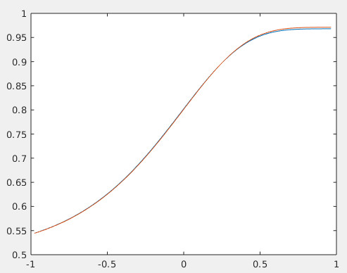Code can also be downloaded here. It runs a psi-method run, then refits the data using PAL_PFHB_Fit, then plots the PFs for each fit (which in this example are virtually identical, see image). They're not exactly the same for reason mentioned above. If you have code like this (but feel free to change anything including using PAL_PFML_Fit instead of PAL_PFHB_modelFit) where the fits are very different, please post here.

rng(0); %Include seed so it will reproduce exactly
NumTrials = 240;
grain = 201;
PF = @PAL_Gumbel; %assumed psychometric function

stimRange = (linspace(PF([0 1 0 0],.1,'inverse'),PF([0 1 0 0],.9999,'inverse'),21));
priorAlphaRange = linspace(PF([0 1 0 0],.1,'inverse'),PF([0 1 0 0],.9999,'inverse'),grain);
priorBetaRange = linspace(log10(.0625),log10(16),grain);
priorGammaRange = 0.5;
priorLambdaRange = 0:.01:.2;

%Initialize PM structure
PM = PAL_AMPM_setupPM('priorAlphaRange',priorAlphaRange,...
'priorBetaRange',priorBetaRange,...
'priorGammaRange',priorGammaRange,...
'priorLambdaRange',priorLambdaRange,...
'numtrials',NumTrials,...
'PF' , PF,...
'stimRange',stimRange);

paramsGen = [0, 1, .5, .02]; %generating parameter values [alpha, beta, gamma, lambda] (or [threshold, slope, guess, lapse])

while PM.stop ~= 1

response = rand(1) < PF(paramsGen, PM.xCurrent); %simulate observer
%update PM based on response:
PM = PAL_AMPM_updatePM(PM,response);

end

data.x = PM.x(1:end-1);
data.y = PM. response;
data.n = ones(size(data.x));
pfhb = PAL_PFHB_fitModel(data,'PF','Gumbel');

plot(priorAlphaRange,PF([PM.threshold(end) 10.^PM.slope(end) PM.guess(end) PM.lapse(end)],priorAlphaRange))
hold on
plot(priorAlphaRange,PF([pfhb.summStats.a.mean 10.^pfhb.summStats.b.mean .5 pfhb.summStats.l.mean],priorAlphaRange))

Thanks for this Nick. Just to check I've understood you – are you saying that although it might be a good idea to refit data collected using Palamedes, this will make very little practical difference? If that's the case, then we will stick to the simpler method of calling PsiObject.thresholdUniformPrior(end), rather than going to the trouble of refitting – close enough is good enough and much less prone to possible errors than refitting (see below...)

However, if I understand correctly, if we were minded to refit the data, then you're saying that because the Psi procedure is a Bayesian method, we should also use a Bayesian fitting procedure? By that logic, I assume that if a Gumbel is used by the Psi procedure during data acquisition, we should also use a Gumbel to fit the data..?

I can't actually see where the estimate of threshold is in your example (there is a plot but no numerical output). To be absolutely sure I am following this properly, below I have set out how I would currently go about pulling out threshold by refitting (bearing in mind I use a Maximum Likelihood fitting method rather than Bayesian and fit with a Cumulative Normal rather than Gumbel; I would potentially change this in future in light of your suggestions):

This code should work for any PsiObject produced using PsiObject = PAL_AMPM<...> methods for a 2AFC task. First, take the data from the PsiObject and arrange it in the manner required by PAL_CumulativeNormal():
Tell the function that we will use Cumulative Normal, and that we are only interested in estimating threshold and slope; guess and lapse rates are fixed:
Next, set up the 'SearchGrid' (which, as I understand it, only provides initial guesses for the free parameters, so ultimately only the values given for gamma and lambda make any difference here; alpha and beta only affect processing time):
Finally, we are ready to fit a model and extract threshold:
...And then we can calculate threshold from the model by finding the value of x where y = 0.76 (76% corresponds to a d-prime of 1). If any of my logic here (or usage of Palamedes) doesn't check out properly, I'd appreciate if you could let me know.

If the PAL_AMPM routines are properly setup there will be very little difference between the estimates it generates and estimates you would get from refitting data with PAL_PFHB routines. But, remember that this thread started off with you noticing discrepancies between estimates reported by PAL_AMPM and estimates reported by a consequent fitting of the data. If that happens I would place more confidence in the estimates reported by consequent fitting. If you refit using PAL_PFHB it is also much easier to check the fit (because it reports diagnostics and you can visually inspect the fit and posteriors using PAL_PFHB_inspectFit and PAL_PFHB_inspectParam, respectively). Also, refitting allows you to fit multiple conditions simultaneously and target interesting research questions directly or implement assumptions.

Yes, for all routines, you should use whatever model for PF (logistic, Gumbel, whatever) you think is closest to the correct model. If that’s the cumulative normal, you should use that in whatever routine you’re using (PAL_AMPM, PAL_PFML, PAL_PFHB, etc.).

Couple of other comments:

There is no need to arrange data in the manner you do before calling PAL_PFML_Fit. After your PAL_AMPM routine finishes (and you set up searchGrid, paramsFree, and assign a function to PF), you can just use this call:
PAL_PFML_Fit will actually arrange the data in the same manner as your code does before performing the fit using an internal call to PAL_PFML_GroupTrialsbyX:
That line of code does the same thing your code does.

‘searchGrid’ does not merely serve to reduce computing time! Likelihood functions may have local maxima. Not using an appropriate searchGrid might result in Nelder-Mead ending up in a local maximum (see here: www.palamedestoolbox.org/understandingfitting.html or here: https://link.springer.com/article/10.37 ... 19-01706-7 for more information).

The ‘76% correct = d-prime of 1’ rule assumes that the observer does not lapse. But the code you give to figure ‘threshold’ using the ‘inverse’ option of PAL_PFML_CumulativeNormal does assume that the observer lapses. In general, we advise against defining ‘threshold’ in terms of the stimulus intensity that corresponds to a particular proportion correct. The generic equation for the PF:



separates the 'perceptual part' [i.e., F(x; ɑ, β)] from the 'decision part'. The perceptual part is what you're interested in. The value you get when using your: is not just a function of the perceptual mechanism, it also depends on what the lapse rate is and how the task happened to be set up (e.g., 2AFC versus 4AFC etc). Let's say you test an observer's ability to, say, detect a stimulus. You use a 2AFC task. Another researcher tests the same observer using the same stimulus but uses a 4AFC task. If you use ɑ as your measure of performance or definition of 'threshold' (we prefer the term 'location parameter' for ɑ over 'threshold' for a multitude of reasons), you and the other researcher should end up with the same estimate (save of course for sampling error). If you use the stimulus intensity that corresponds to a particular proportion correct, you will not. If you retest your observer, again using a 2AFC task but now when they're distracted by something (i.e., their lapse rates differ between the two occasions) you will end up with the same estimate for ɑ (save for sampling error and assuming you successfully estimate the lapse rate in both situations), but your estimates for 'threshold' defined in terms of intensity at which observer x% correct will differ.

Another reason for using location parameter ɑ as your measure of performance over one based on proportion correct: PAL_AMPM is set up to optimize the estimate of the location parameter. It makes sense to use the parameter that you optimized as your parameter of interest over a parameter that wasn't optimized. Also, the standard error or credible interval on a threshold based on proportion correct can give you a false sense of precision with which the 'perceptual part' of the psychometric function was estimated. Very counterintuitively, you can have a much smaller standard error (or credible interval) on a threshold defined in terms of proportion correct as compared to the standard error (or credible interval) on the location parameter (see here: https://www.palamedestoolbox.org/parame ... dancy.html for dramatic example).