
How to Perform a Model Comparison
Whether you prefer using Maximum-Likelihood methods (e.g., PAL_PFML_fit, PAL_PFLR_ModelComparison) or Bayesian methods (e.g., PAL_PFHB_fitModel), figuring out whether
some experimental manipulation affects, say, the location parameter ('threshold') of a psychometric function can be done by an appropriate reparameterization of your model.
Let's go over a simple single-subject, two-condition experiment. Figure 1 shows the data with the fits we derived with:
>>data.x = [-2:1:2, -2:1:2];
>>data.y = [62 73 84 93 99 55 68 75 91 98];
>>data.n = 100*ones(size(data.x));
>>data.c = [1 1 1 1 1 2 2 2 2 2] ;
>>pfhb_unreparam = PAL_PFHB_fitModel(data);
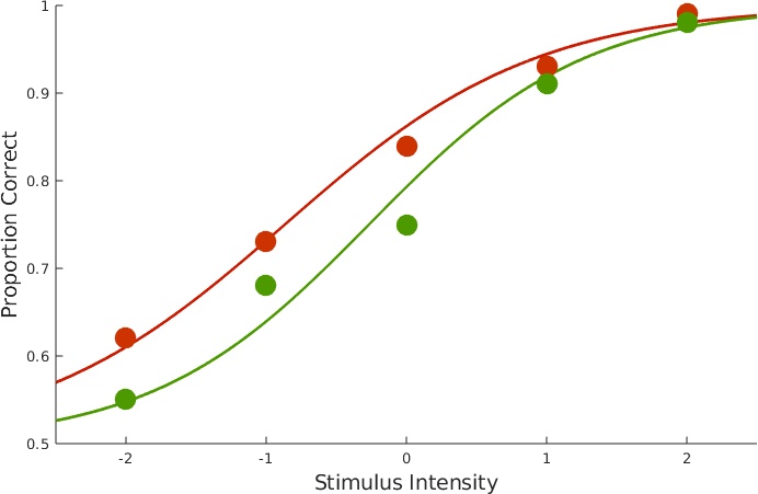 Figure 1. Data with fits.
The above figure was custom-created for this page, but you can obtain plots for data and fit for individual conditions using PAL_PFHB_inspectFit(pfhb_unreparam,'all'). We can get an overview of parameter estimates by calling:
>>PAL_PFHB_drawViolins(pfhb_unreparam)
which produces Figure 2. It's not immediately obvious whether the difference between the location parameters in condition 1 and 2 is sufficient to infer a 'real' effect.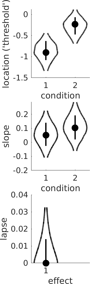 Figure 2. Violin plots. Dots show mode in the marginal posterior distribution, lines show 68% credible intervals, and curves show the marginal posterior distribution across its 95% credible interval. Is there sufficient evidence to conclude that location parameters differ between conditions?
We can get a clearer picture by reparameterizing the location parameters such that we can directly evaluate the difference between the location parameters. We can do this using a model matrix:
Figure 2. Violin plots. Dots show mode in the marginal posterior distribution, lines show 68% credible intervals, and curves show the marginal posterior distribution across its 95% credible interval. Is there sufficient evidence to conclude that location parameters differ between conditions?
We can get a clearer picture by reparameterizing the location parameters such that we can directly evaluate the difference between the location parameters. We can do this using a model matrix:
M = [1 1; 1 -1];
Each row defines a new parameter as a linear combination of the location thresholds. The first row [1 1] defines a new parameter as the sum of the location parameters:
sum = (1)*(location parameter in condition 1)+(1)*(location parameter in condition 2).
The second row [1 -1] defines a second parameter as the difference between the location parameters:
difference = (1)*(location parameter in condition 1)+(-1)*(location parameter in condition 2). Learn more about model matrices and how to design and use them to target specific research questions on our model matrices page. We can now run the analysis like this:
>>pfhb_reparam = PAL_PFHB_fitModel(data, 'a', M);
>>PAL_PFHB_drawViolins(pfhb_reparam)
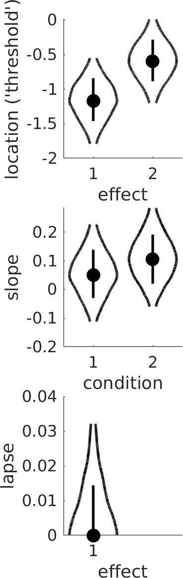 Figure 2. Violin plot showing posterior distributions for reparameterized location parameters.
Note that the location parameters are now labeled 'effects' in the plot since the parameters shown do not correspond directly to the location parameters but rather to the sum and difference
parameters defined by the model matrix M. Thus, in order to evaluate the experimental effect we are here not comparing the two violins, but rather we evaluate whether the value 0 seems credible for
the 'difference parameter' (labeled as effect 2 in the Figure). From Figure 2, it seems clearer that there is likely a real difference in thresholds between the two conditions. Note that a more
detailed view of the posterior distribution for the difference parameter can be obtained like this:
Figure 2. Violin plot showing posterior distributions for reparameterized location parameters.
Note that the location parameters are now labeled 'effects' in the plot since the parameters shown do not correspond directly to the location parameters but rather to the sum and difference
parameters defined by the model matrix M. Thus, in order to evaluate the experimental effect we are here not comparing the two violins, but rather we evaluate whether the value 0 seems credible for
the 'difference parameter' (labeled as effect 2 in the Figure). From Figure 2, it seems clearer that there is likely a real difference in thresholds between the two conditions. Note that a more
detailed view of the posterior distribution for the difference parameter can be obtained like this:
>>PAL_PFHB_inspectParam(pfhb_reparam, 'a', 'effect', 2);
Note that a posterior for the difference between any pair of parameters (compare to a 'pairwise comparison' after, say, an ANOVA) can also be derived if no reparameterization was used in the analysis using the PAL_PFHB_inspectParam routine. The following calls should lead to (approximately) the same posterior as the previous call:
>>PAL_PFHB_inspectParam(pfhb_unreparam, 'a', 'condition', 1, 'a', 'condition', 2); %Note that we're passing the unreparameterized model structure
The difference between the location parameters in the two conditions can also be evaluated by a traditional Null Hypothesis Significance Test using the so-called likelihood ratio test. This approach is outlined in detail in our 2018 paper that can be accessed here: Prins & Kingdom (2018). This approach is also demonstrated in the routine PAL_PFLR_Demo (and others) in the PalamedesDemos folder.
>>data.x = [-2:1:2, -2:1:2];
>>data.y = [62 73 84 93 99 55 68 75 91 98];
>>data.n = 100*ones(size(data.x));
>>data.c = [1 1 1 1 1 2 2 2 2 2] ;
>>pfhb_unreparam = PAL_PFHB_fitModel(data);
Figure 1. Data with fits.
The above figure was custom-created for this page, but you can obtain plots for data and fit for individual conditions using PAL_PFHB_inspectFit(pfhb_unreparam,'all'). We can get an overview of parameter estimates by calling:
>>PAL_PFHB_drawViolins(pfhb_unreparam)
which produces Figure 2. It's not immediately obvious whether the difference between the location parameters in condition 1 and 2 is sufficient to infer a 'real' effect.
Figure 2. Violin plots. Dots show mode in the marginal posterior distribution, lines show 68% credible intervals, and curves show the marginal posterior distribution across its 95% credible interval. Is there sufficient evidence to conclude that location parameters differ between conditions?
We can get a clearer picture by reparameterizing the location parameters such that we can directly evaluate the difference between the location parameters. We can do this using a model matrix:M = [1 1; 1 -1];
Each row defines a new parameter as a linear combination of the location thresholds. The first row [1 1] defines a new parameter as the sum of the location parameters:
sum = (1)*(location parameter in condition 1)+(1)*(location parameter in condition 2).
The second row [1 -1] defines a second parameter as the difference between the location parameters:
difference = (1)*(location parameter in condition 1)+(-1)*(location parameter in condition 2). Learn more about model matrices and how to design and use them to target specific research questions on our model matrices page. We can now run the analysis like this:
>>pfhb_reparam = PAL_PFHB_fitModel(data, 'a', M);
>>PAL_PFHB_drawViolins(pfhb_reparam)
Figure 2. Violin plot showing posterior distributions for reparameterized location parameters.
Note that the location parameters are now labeled 'effects' in the plot since the parameters shown do not correspond directly to the location parameters but rather to the sum and difference
parameters defined by the model matrix M. Thus, in order to evaluate the experimental effect we are here not comparing the two violins, but rather we evaluate whether the value 0 seems credible for
the 'difference parameter' (labeled as effect 2 in the Figure). From Figure 2, it seems clearer that there is likely a real difference in thresholds between the two conditions. Note that a more
detailed view of the posterior distribution for the difference parameter can be obtained like this:>>PAL_PFHB_inspectParam(pfhb_reparam, 'a', 'effect', 2);
Note that a posterior for the difference between any pair of parameters (compare to a 'pairwise comparison' after, say, an ANOVA) can also be derived if no reparameterization was used in the analysis using the PAL_PFHB_inspectParam routine. The following calls should lead to (approximately) the same posterior as the previous call:
>>PAL_PFHB_inspectParam(pfhb_unreparam, 'a', 'condition', 1, 'a', 'condition', 2); %Note that we're passing the unreparameterized model structure
The difference between the location parameters in the two conditions can also be evaluated by a traditional Null Hypothesis Significance Test using the so-called likelihood ratio test. This approach is outlined in detail in our 2018 paper that can be accessed here: Prins & Kingdom (2018). This approach is also demonstrated in the routine PAL_PFLR_Demo (and others) in the PalamedesDemos folder.
Beyond Pairwise Comparisons
Let's say you do an experiment with four conditions and the conditions vary with respect to some quantitative variable (spatial frequency, contrast, viewing distance, whatever). Figure 3 shows the
data with the fits obtained by:
>>data.x = [-2:1:2, -2:1:2, -2:1:2, -2:1:2];
>>data.y = [84 92 128 137 143 67 85 103 131 139 73 85 92 125 143 82 86 97 122 141];
>>data.n = 150*ones(size(data.x));
>>data.c = [1 1 1 1 1 2 2 2 2 2 3 3 3 3 3 4 4 4 4 4] ;
>>pfhb_unreparam = PAL_PFHB_fitModel(data);
>>PAL_PFHB_drawViolins(pfhb_unreparam);
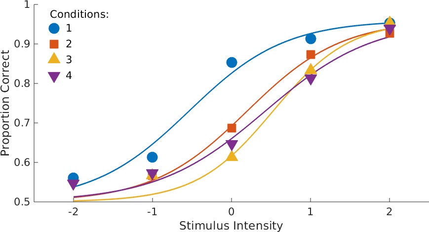 Figure 3. Data with fits. This figure custom-created for this page, but you can obtain plots for data with fit for individual conditions using
PAL_PFHB_inspectFit(pfhb_unreparam,'all')
Figure 3. Data with fits. This figure custom-created for this page, but you can obtain plots for data with fit for individual conditions using
PAL_PFHB_inspectFit(pfhb_unreparam,'all')
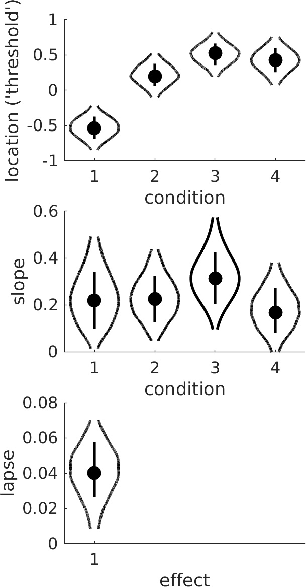 Figure 4. Violins.
From the violin plots it seems that the slope is not affected by condition but that the location parameter increases with condition. It also seems that the increase in location parameter levels off
as condition increases. Is there sufficient evidence that the increase deviates from linear? This question calls for a trend analysis. The routine PAL_Contrasts can generate a Model Matrix that
reparameterizes the location thresholds into polynomial trends.
Figure 4. Violins.
From the violin plots it seems that the slope is not affected by condition but that the location parameter increases with condition. It also seems that the increase in location parameter levels off
as condition increases. Is there sufficient evidence that the increase deviates from linear? This question calls for a trend analysis. The routine PAL_Contrasts can generate a Model Matrix that
reparameterizes the location thresholds into polynomial trends.
>>M = PAL_Contrasts(4,'polynomial');
>>pfhb_reparam = PAL_PFHB_fitModel(data, 'a', M, 'b', 'constrained);
>>PAL_PFHB_drawViolins(pfhb_reparam);
Note that since slope does not seem to be affected by condition, we chose to reduce model complexity by imposing the constraint that slopes are equal in the conditions (good models have few parameters). The four 'effects' shown for the location parameter correspond to the 'intercept' (sum of location parameters across condition), linear trend (does location tend to increase or decrease with condition?), quadratic trend (does the line relating location to condition need a bend?), and cubic trend (does it need two bends?), respectively. Not surprisingly, the linear trend ('effect 2' in violin plot) is unlikely to equal 0. It also seems that the quadratic trend ('effect 3') is not likely to equal 0, so it appears the bend is 'real'.
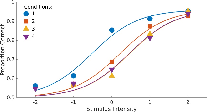 Figure 5. Data with fits. Note that the four functions now have equal slopes as specified in the call to PAL_PFHB_fitModel.
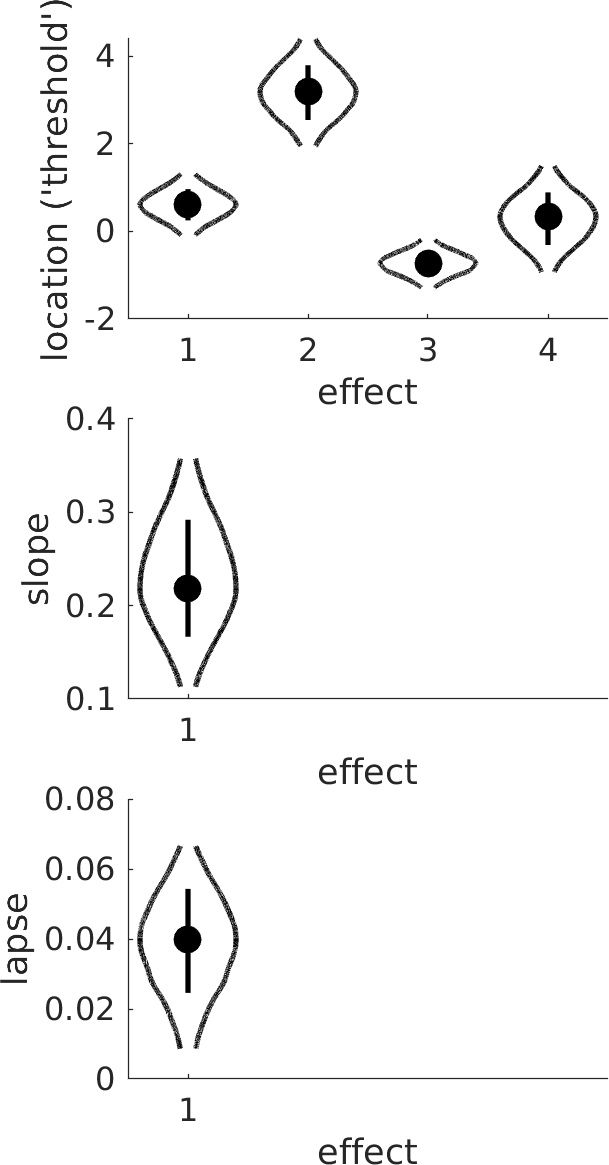 Figure 6. Violins.
A more traditional Null Hypothesis Test approach to these data is performed by PAL_PFLR_FourGroup_Demo in the PalamedesDemos folder.
Figure 6. Violins.
A more traditional Null Hypothesis Test approach to these data is performed by PAL_PFLR_FourGroup_Demo in the PalamedesDemos folder.
>>data.x = [-2:1:2, -2:1:2, -2:1:2, -2:1:2];
>>data.y = [84 92 128 137 143 67 85 103 131 139 73 85 92 125 143 82 86 97 122 141];
>>data.n = 150*ones(size(data.x));
>>data.c = [1 1 1 1 1 2 2 2 2 2 3 3 3 3 3 4 4 4 4 4] ;
>>pfhb_unreparam = PAL_PFHB_fitModel(data);
>>PAL_PFHB_drawViolins(pfhb_unreparam);
Figure 3. Data with fits. This figure custom-created for this page, but you can obtain plots for data with fit for individual conditions using
PAL_PFHB_inspectFit(pfhb_unreparam,'all')
Figure 4. Violins.
>>M = PAL_Contrasts(4,'polynomial');
>>pfhb_reparam = PAL_PFHB_fitModel(data, 'a', M, 'b', 'constrained);
>>PAL_PFHB_drawViolins(pfhb_reparam);
Note that since slope does not seem to be affected by condition, we chose to reduce model complexity by imposing the constraint that slopes are equal in the conditions (good models have few parameters). The four 'effects' shown for the location parameter correspond to the 'intercept' (sum of location parameters across condition), linear trend (does location tend to increase or decrease with condition?), quadratic trend (does the line relating location to condition need a bend?), and cubic trend (does it need two bends?), respectively. Not surprisingly, the linear trend ('effect 2' in violin plot) is unlikely to equal 0. It also seems that the quadratic trend ('effect 3') is not likely to equal 0, so it appears the bend is 'real'.
Figure 5. Data with fits. Note that the four functions now have equal slopes as specified in the call to PAL_PFHB_fitModel.
Figure 6. Violins.
More examples
Conditions differ with respect to more than one variable? Interested to see whether the variables interact in their effect on location (or slope or lapse rate or guess rate)? We can do that.
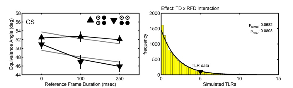
The figure below show data from one observer in Prins (2008; Correspondence matching in long-range apparent motion precedes featural analysis. Perception, 37, 1022-1036). The figure shows the location parameters (PSEs) of psychometric functions in 6 conditions in a 2 ('Token Distribution'; TD) x 3 ('Reference Frame Duration'; RFD) design. Model matrices were used to define and compare two models, one of which allowed TD and RFD to interact (black lines in graph), the other of which did not allow them to interact (gray lines).
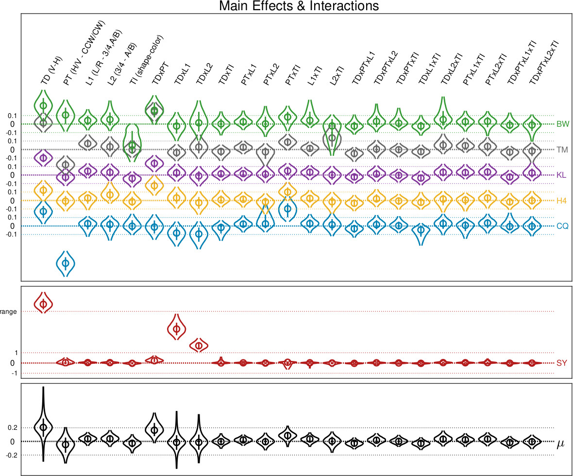
 You have more IVs? Sure. The figure below taken from Prins, Behavior Research Methods, 2023. It shows estimates of 23 parameters corresponding to main and interaction effects on location parameter
for six observers in a 2 x 2 x 2 x 3 factorial design (observer SY shown on separate graph due to being an atypical observer). Bottom graph shows corresponding hyper-parameters.
You have more IVs? Sure. The figure below taken from Prins, Behavior Research Methods, 2023. It shows estimates of 23 parameters corresponding to main and interaction effects on location parameter
for six observers in a 2 x 2 x 2 x 3 factorial design (observer SY shown on separate graph due to being an atypical observer). Bottom graph shows corresponding hyper-parameters.
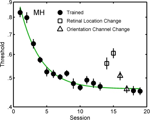
 In the figure below the symbols show individual fits for all sessions in a perceptual learning experiment Prins & Streeter, Vision Sciences Society, 2009. Two models of these data are compared by PAL_PFLR_LearningCurve_Demo. In the more elaborate
('fuller') of the two models the sessions shown with solid symbols are constrained to follow a (three parameter) exponential decay function, while the open symbols were unconstrained. The lesser
model was identical to the fuller except that all but the open square symbols were constrained to follow an exponential decay function. Such a comparison answers the question: do the open triangles
deviate significantly from the learning curve?
In the figure below the symbols show individual fits for all sessions in a perceptual learning experiment Prins & Streeter, Vision Sciences Society, 2009. Two models of these data are compared by PAL_PFLR_LearningCurve_Demo. In the more elaborate
('fuller') of the two models the sessions shown with solid symbols are constrained to follow a (three parameter) exponential decay function, while the open symbols were unconstrained. The lesser
model was identical to the fuller except that all but the open square symbols were constrained to follow an exponential decay function. Such a comparison answers the question: do the open triangles
deviate significantly from the learning curve?
The figure below show data from one observer in Prins (2008; Correspondence matching in long-range apparent motion precedes featural analysis. Perception, 37, 1022-1036). The figure shows the location parameters (PSEs) of psychometric functions in 6 conditions in a 2 ('Token Distribution'; TD) x 3 ('Reference Frame Duration'; RFD) design. Model matrices were used to define and compare two models, one of which allowed TD and RFD to interact (black lines in graph), the other of which did not allow them to interact (gray lines).
You have more IVs? Sure. The figure below taken from Prins, Behavior Research Methods, 2023. It shows estimates of 23 parameters corresponding to main and interaction effects on location parameter
for six observers in a 2 x 2 x 2 x 3 factorial design (observer SY shown on separate graph due to being an atypical observer). Bottom graph shows corresponding hyper-parameters.
In the figure below the symbols show individual fits for all sessions in a perceptual learning experiment Prins & Streeter, Vision Sciences Society, 2009. Two models of these data are compared by PAL_PFLR_LearningCurve_Demo. In the more elaborate
('fuller') of the two models the sessions shown with solid symbols are constrained to follow a (three parameter) exponential decay function, while the open symbols were unconstrained. The lesser
model was identical to the fuller except that all but the open square symbols were constrained to follow an exponential decay function. Such a comparison answers the question: do the open triangles
deviate significantly from the learning curve?