
The Palamedes PFML routines fit psychometric functions (PFs) using a maximum likelihood criterion. Simply put, what that means is that, of all possible PFs (i.e., all combinations of possible values for the free parameters), it finds that PF that has the highest probability of generating the exact same responses to the stimuli that your observer generated. Unfortunately, there is no analytical way in which to do this. Instead, Palamedes has to perform a search for this best-fitting PF. This turns out to be tricky. There are an infinite number of candidates to consider! Not to worry, Palamedes will find the function that maximizes the likelihood. But unfortunately, this may not always be a function you expected or like to get. Understanding how maximum likelihood fitting works and why sometimes you get results you do not like will help you get better fits and avoid mistakes. We'll explain by example.
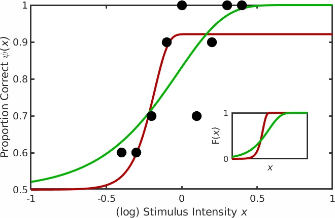
Figure 1.
Figure 2. Nelder-Mead finds a maximum.
The simplex will never make it to the exact position of the highest point on the hill but it can get arbitrarily close to it. The decision to stop the search is based on the size of the simplex and is set using 'tolerance' values. There are actually two tolerance values involved, one ('TolX') has to do with the values of the parameters, the other ('TolFun') has to do with the likelihood values. Simply put, the search stops when all feet of the tripod are no farther than the value of TolX from the best foot in either the location direction or the slope direction (measured in whatever units location and slope are measured in) AND the log likelihood associated with the worst foot is no farther than the value of TolFun below the log likelihood associated with the best foot. In other words, when the simplex is visualized in three dimensions with the third dimension corresponding to the value to be maximized, the search stops once the simplex fits in a box with length and width no larger than TolX and a height no more than TolFun. Both TolX and TolFun are, by default, set to 1e-6 (0.000001) in Palamedes. Once the tolerance criteria have been met the search stops and the location and slope values corresponding to the position of the best foot are reported as the parameter estimates. The solution converged on using the above strategy is the green curve in Figure 1. Code snippet 1 (click link at bottom of page to download code snippets, code Snippets require Palamedes) performs the fit described above starting at the same initial position of the vertex as shown in Figure 2 (note though that after the 23 iterations shown in Figure 2, tolerance values have not been met and more iterations are performed in code snippet 1 than are shown in Figure 2). This principle will readily generalize to higher dimensional parameter spaces. For example, let's say you read somewhere that you should allow the lapse rate to vary when you fit a PF. You now have three parameters to estimate (location, slope and lapse rate). Nelder-Mead will work, in principle, for parameter spaces of any dimension. The simplex will always have n + 1 verteces for an n-dimensional parameter space. A graphical representation of the three dimensional (location x slope x lapse rate) likelihood function for the data in Figure 1 is given in Figure 3.
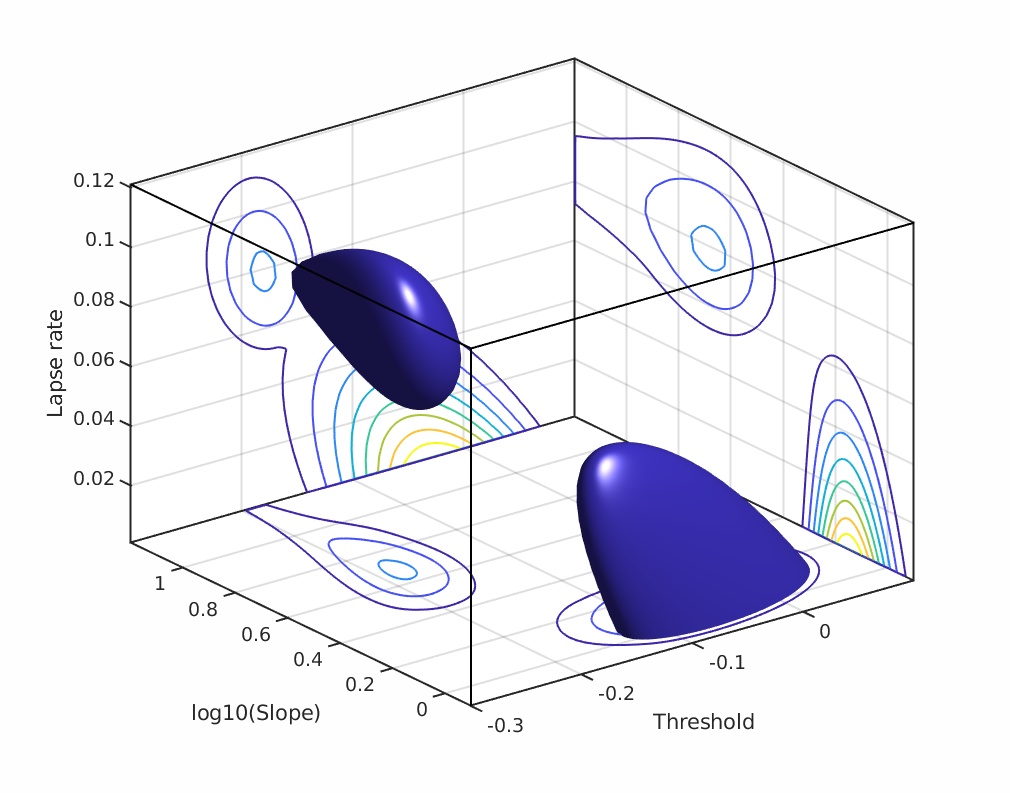
Figure 3. Local maximum.
Thus, in order to avoid ending up in a local maximum, it is important that we find a starting position for our simplex that is on the hillside of the highest hill in the likelihood space. One way in which to do this is to find a starting position by first performing a 'brute force' search through a grid defined across the parameter space. The grid is defined by specifying a range of values for all of the free parameters. Likelihood values are then calculated for all combinations of parameter values contained in the grid. The combination with the highest likelihood serves as the starting point for the simplex. Lucky for us, today's computers can perform a brute force search through a finely spaced search grid in a very short period of time. For example, the (very modest) laptop at which this is written, just performed a brute force search through this grid: searchGrid.alpha = -.4:.005:.4, searchGrid.beta = 10.^[-1:.025:2], searchGrid.lambda = [0:.01:.15] in about 2/3 of a second. There are a total of 311,696 PFs in this grid (55,809 of which are contained in the space shown in Figure 3). Code snippet 2 performs the fit as described above.
Note that the search grid that searches for a starting point for a simplex should include all the free parameters that will be considered by the simplex search. For example, the lesser heat source shown in Figure 3 will have a higher likelihood than the greater heat source when we fix the lapse rate at 0.06. Thus, a brute force search through location and slope values that uses a fixed value of 0.06 for the lapse rate would result in an initial position for the simplex near the lesser heat source. A subsequent simplex search that includes the lapse rate but starts at the initial position we found while fixing the lapse rate at 0.06 would then converge on the maximum value in the lesser heat source. This is demonstrated in code snippet 3.
Sometimes, however, the Nelder-Mead algorithm will report that it failed to converge. It may also sometimes report that it converged successfully when in fact it hasn't. If either of these happens, Nelder-Mead may report parameter estimates that are nowhere near those expected. Under what circumstances might this happen?
Figure 4 shows some hypothetical data from a 2 AFC experiment. There were 5 stimulus intensities used with 10 trials at each of these intensities. Using PAL_PFML_Fit to perform a simplex search for a location value and a slope value while keeping the guess and lapse rates fixed (we used 0.5 and 0.03 respectively) will not converge. The simplex search will chase after a maximum in the likelihood function but will not find one. After a criterion number of iterations and/or function evaluations (the default is 800 for each when searching for two parameters), the simplex gives up on finding a maximum, and in Palamedes version 1.9.0 or lower PAL_PFML_Fit would set the 'exitflag' to zero to let you know about it. The parameter values it returned for this specific problem are -4550.9613 for the location and 0.000035559 for the slope (Palamedes behaves differently now, but you can still have Palamedes do this old-style: see code snippet 4). These numbers seem outrageous and arbitrary. However, keep in mind that the Gumbel is a monotonically increasing function of the data, but that the data follow an overall downward trend! As we will argue, Palamedes failed to find a maximum because there was no maximum to be found! The data do not support the estimation of a location and a slope. The seemingly outrageous and arbitrary fit of Palamedes is a typical case of 'garbage in, garbage out'. Or is it?
The green horizontal line in Figure 4 which has a value of 0.86 (the overall proportion correct across all 50 trials) is actually not a horizontal line. It is actually (a tiny part of) a very, very shallow Gumbel function! If by now you guessed that it is a Gumbel with location equal to -4550.9613 and slope equal to 0.000035559 (guess rate = 0.5, and lapse rate = 0.03) you are right. The parameter estimates Palamedes reported are not arbitrary at all! Even more, from a purely statistical perspective they are not outrageous either! Palamedes is asymptotically near fitting a horizontal line at the observed overall proportion correct observed. This is the best fit that can be obtained given the constraint that a Gumbel needs to be fitted. Note that there is indeed no maximum in the likelihood function. The line shown in Figure 4 can always be made a little straighter and more horizontal by moving the location to an even lower value and adjusting the slope value such that, within the stimulus intensity range, the function has values that are asymptotically close to 0.86. Starting with Palamedes version 1.9.1, Palamedes will figure out that no maximum in the likelihood function exists and will also figure out which limiting function Nelder-Mead is chasing after but will never (exactly) reach even though it can get arbitrary close to it. The limiting function will be either a constant function as in this example or a step function (see below). Palamedes will also assign values to parameter estimates (though not all these values may be finite). In this example, Palamedes assigns a 'value' of -Inf to the location parameter and a value of 0 to the slope parameter. These values correspond to those Nelder-Mead was chasing after.
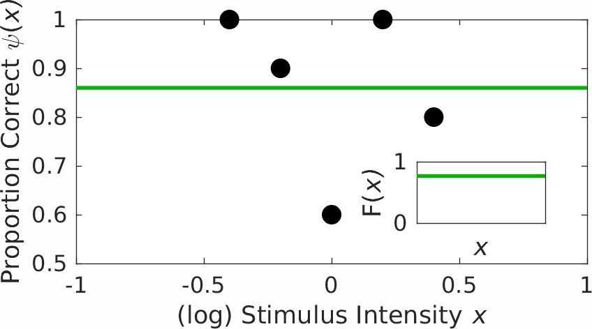
Figure 4. Example of what Prins (2019) and Palamedes label 'scenario -3'.
Any researcher who obtains the data shown in Figure 4 (and plots them and looks at them!) will readily understand that PAL_PFML_Fit will not give a fit with values for the location and slope that the researcher might have expected. It is a little harder to see why problems arise when the data look fine (say 6, 8, 8, 10, 9 correct responses, respectively, for the 5 stimulus levels, each again out of 10 trials). Even though the fit to these data is fine (location = -0.1040, slope = 1.836, code snippet 5), finding a standard error using a bootstrap routine or determining the goodness of fit using Monte Carlo simulations leads to poor results (specifically: warnings from Palamedes stating that not all simulations converged combined with reported NaNs ('not a number') estimates for standard errors of location and slope parameters (code snippet 5). The problem is that some of the simulations performed during the bootstrap will result in simulated data such as those shown in Figure 4, resulting in failures of convergence and parameter estimates that are equal to Inf or -Inf. The standard error that a routine such as PAL_PFML_BootstrapParametric produces is just the standard deviation of the parameter estimates resulting from the simulations and they can not be calculated when some values are non-finite.
A distinct advantage of figuring out which limiting function (constant or step) Palamedes is trying to approach when no true maximum exists is that meaningful log-likelihood values can be derived even when no true maximum in the likelihood function exists. The log likelihood value of the limiting function can be approached by the PF to any arbitrary degree of precision. Thus, these values can then be used to determine a Monte Carlo based p-value for a Goodness-of-Fit test even though not all Monte Carlo simulations may have a true maximum in the likelihood function. This is demonstrated in code snippet 5 also.
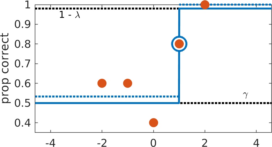
Figure 5. Example of what Prins (2019) and Palamedes label 'scenario -1'. Think you can spot these by eye? Take a stab at some here.
Figure 6 shows what we label scenario -2. It is similar to scenario -1 except there is no specific stimulus intensity that the function will attempt to match exactly. In the example in Figure 6, the location parameter will have some value between -1 and 0 while the slope again will tend towards infinity. The broken lines again show what would happen if the guess and/or lapse rate were freed.
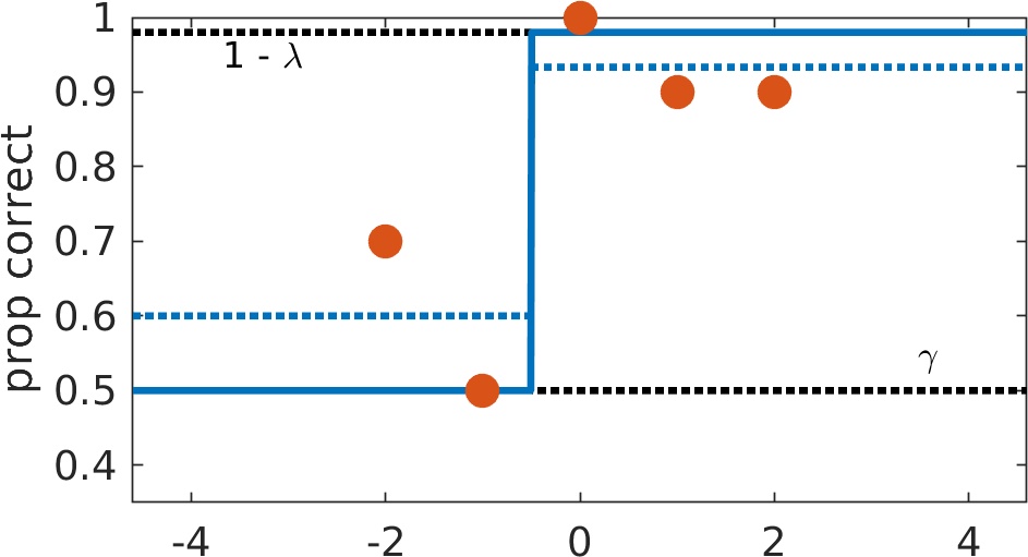
Figure 6. Example of what Prins (2019) and Palamedes label 'scenario -2'. Think you can spot these by eye? Take a stab at some here.
Note that some software packages may 'fail to fail' and will happily report nice-looking estimates of your parameters and their standard errors even if your data do not support these estimates. This is frustrating for us, because it seems as if Palamedes fails where other packages seem to succeed. When Palamedes fails to fit some data while another package appears to fit those data just fine, we encourage you to compare the log-likelihood values of the fit between the two packages and also to inspect how the fitted functions compare to your data (which is good practice anyway).
We regularly receive questions from users regarding failed fits and it is almost universally the case that the user simply did not have sufficient data to estimate the parameters they were attempting to estimate. A key consideration is that freeing more parameters does not necessarily make a model a better model (remember Occam's razor: a good model has few parameters). The solution here is to make sure that you have sufficient data to support estimation of the model that you wish to fit. In other words: either get more data or use a fixed value for the parameters regarding which you do not have sufficient information in your data. By way of demonstration, code snippet 6 refits the data of code snippet 5 but this time using a fixed value for the slope. It successfully estimates the location, generates a standard error for the location estimate and determines the goodness-of-fit for the overall fit of this model. Even the data shown in Figure 4 allow estimation of a location (with a standard error) and a goodness-of-fit of the resulting model. If you use a fixed slope in your fit, it might be best to avoid a parametric bootstrap (use the nonparametric bootstrap instead). If you do perform a parametric bootstrap, it is pertinent that you use a value for the slope that is realistic: the value for the SE on the location will, in some circumstances, be determined entirely by the value for the slope that you use.
- Rule number one: Don't estimate parameters unless your data contain sufficient information to allow their estimation. Rather, fix them (or get more data).
- Make sure to select parameter ranges for the search grid that are wide enough to contain the PF associated with the (absolute) maximum likelihood. To this end, plot some PFs with various locations and slopes to determine what range of values to include in the search grid.
- Know your Gumbel from your Weibull! (see here: www.palamedestoolbox.org/weibullandfriends.html). Also know, say, your Logistic from your Quick. Etc. For example, a Logistic with beta = 1.5 has a very different steepness compared to a Quick with beta = 1.5.
- Space slope values in the searchGrid on a log scale (but provide their values in linear units). Use something like: searchGrid.beta = 10.^[-1:.1:2];
- If you follow an adaptive method with an ML fit, do not free parameters that were not targeted by the adaptive method (e.g., if you use an up/down method do not estimate the slope in subsequent ML fit, if you use the original psi method (Kontsevich & Tyler, 1999) do not free the lapse rate in a subsequent ML fit).
- In case a fit fails to converge, increasing the maximum number of iterations and function evaluations allowed might help [see code snippet 7 on how to increase these values or refer to help section of a function such as PAL_PFML_Fit (type 'help PAL_PFML_Fit')]. Note though that your likelihood function may not contain a maximum in which case this (or any other) strategy will not work.
- You can increase the precision of parameter estimates by changing the tolerance values using the 'searchOptions' argument of a function such as PAL_PFML_Fit. Reducing tolerance values (i.e., increasing precision) might require you to increase the maximum number of iterations and/or function evaluations allowed also. See code snippet 7.
Nelder, J.A. & Mead, R. (1965). A simplex method for function minimization. Computer Journal, 7, 308-313.
Prins, N. (2019). Too much model, too little data: How a maximum-likelihood fit of a psychometric function may fail and how to detect and avoid this. Attention, Perception, & Psychophysics. https://doi.org/10.3758/s13414-019-01706-7