- Palamedes centers prior for location ('threshold') parameter(s) on the stimulus intensities used during testing.
- Palamedes centers prior for log10(slope) parameter(s) under the assumption that the stimulus intensities used during testing cover much of the dynamic range of the psychometric function (PF).
- Priors for the guess rate and lapse rate are not dependent on stimulus placement.
- Default priors are very wide (i.e., not very informative). If you have 'Too much model, too little data' (see Prins, 2019), your likelihood function is probably a mess (see our page on maximum likelihood fitting) and you will likely have to narrow the priors in order for the analysis to converge.
- Importantly, when multiple conditions and/or subjects are combined in single analysis, identical priors will be applied across all conditions/subjects even if different stimulus placements were used. This ensures that any differences between posteriors are the result of differences in responses/behavior, not differences in priors.
- Remember that you can always provide your own priors, overriding those that Palamedes came up with. We won't be offended.
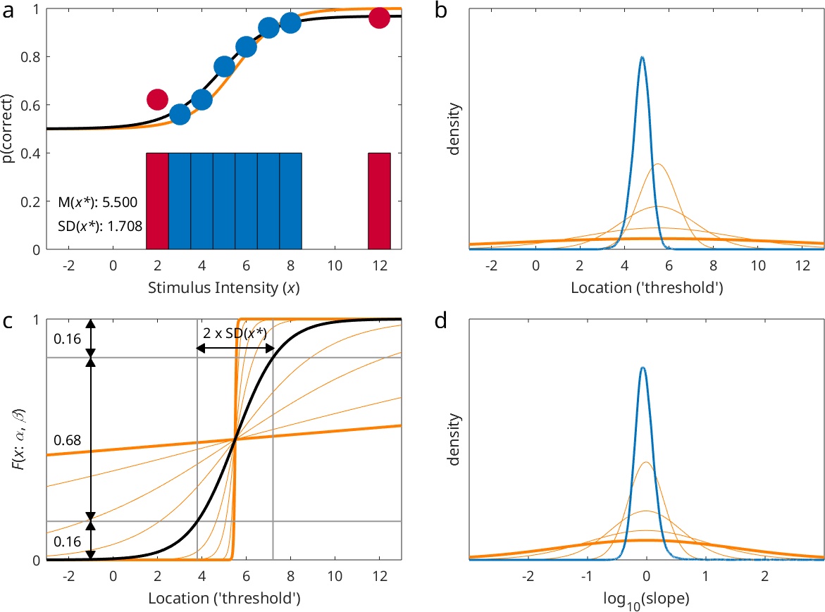 Figure 1. See text for details.
The mean and standard deviation of the trimmed intensities are given in Figure 1a as M(x*) and SD(x*), respectively. The mean of the prior distribution for the location ('threshold') parameter
is set to the mean of the trimmed stimulus intensities M(x*) used in the experiment (here: 5.500). By default, the standard deviation of the prior distribution for the location threshold is set
to four times the standard deviation of the stimulus intensities used (here: 4 x 1.708 = 6.832). The resulting prior distribution for this experiment is shown in Figure 1b by the thick orange
line. Note that this prior is near uniform within the entire stimulus range used in the experiment (i.e., it is a relatively non-informative prior). We call the multiplicative factor on the sd
of the prior the prior width factor for the location parameter and it may be changed from the default value (4) by the user. The light orange lines in Figure 1b show priors using location prior width
factors of .5, 1, and 2. The blue distribution in Figure 1b shows the posterior distribution for the location parameter when the default value of 4 was used for the location prior width factor.
The mean of the prior distribution for the log10(slope) parameter is chosen such that the middle 68% of the range of F(x; α, β) (see equation 1) corresponds to a width equal to twice
the standard deviation of the (trimmed) stimulus intensities [SD(x*)] used in the experiment (see Figure 1c).
Figure 1. See text for details.
The mean and standard deviation of the trimmed intensities are given in Figure 1a as M(x*) and SD(x*), respectively. The mean of the prior distribution for the location ('threshold') parameter
is set to the mean of the trimmed stimulus intensities M(x*) used in the experiment (here: 5.500). By default, the standard deviation of the prior distribution for the location threshold is set
to four times the standard deviation of the stimulus intensities used (here: 4 x 1.708 = 6.832). The resulting prior distribution for this experiment is shown in Figure 1b by the thick orange
line. Note that this prior is near uniform within the entire stimulus range used in the experiment (i.e., it is a relatively non-informative prior). We call the multiplicative factor on the sd
of the prior the prior width factor for the location parameter and it may be changed from the default value (4) by the user. The light orange lines in Figure 1b show priors using location prior width
factors of .5, 1, and 2. The blue distribution in Figure 1b shows the posterior distribution for the location parameter when the default value of 4 was used for the location prior width factor.
The mean of the prior distribution for the log10(slope) parameter is chosen such that the middle 68% of the range of F(x; α, β) (see equation 1) corresponds to a width equal to twice
the standard deviation of the (trimmed) stimulus intensities [SD(x*)] used in the experiment (see Figure 1c).
Equation 1: 
The curve shown in black in Figure 1c corresponds to F(x; α, β) with alpha and beta parameters corresponding to the means of the prior distributions for the location and log10(slope) parameters. Note that for the normal distribution, the mean, median, and mode are equal. In other words, this curve is, based on the placement of stimuli, considered to be the most likely model for F(x; α, β). The standard deviation for the prior on the log10(slope) parameter is by default set to 1.5. We refer to the standard deviation of this prior as the prior width factor for the slope parameter. Remember that, since the slope parameter is the log10 transform of the 'raw' slope parameter (β in equation 1), each unit difference in the log10(slope) parameter corresponds to an order of magnitude difference in the 'raw' slope and the 'width' of the PF. Thus, one standard deviation of the prior distribution away from the mean corresponds to a function that is 101.5 = 31.6 times as wide (or narrow) relative to the PF that is at the mean and mode of the prior. The thick orange curves in Figure 1c show PFs with log10(slope) values that are 1.5 units away from the prior's mean value. From this, it is clear that the default prior on log10(slope) also is not very informative. The user can change the informativeness of the prior by choosing a different value for the prior width factor for the slope parameter. The thin orange curves in Figure 1c show PFs with log10(slope) values that are 0.3, 0.6, and 1 removed from the curve shown in black. These would correspond to PFs that are 100.3 (≈ 2), 100.6 (≈ 4), and 101 (= 10) times as steep/narrow or shallow/wide as the black curve. Figure 1d shows the corresponding prior distributions. The blue curve shows the posterior distribution for the log10(slope) parameter based on the analysis. The orange curve in Figure 1a shows a PF with α, β, and λ values that correspond to the modes in the respective prior distributions.
When the analysis includes multiple conditions and/or subjects: In the case of an analysis in which multiple conditions and/or subjects are included, the values for the priors are based on the intensities used in all condition/subject combinations. Importantly, the same prior will then be applied to all conditions and subjects in the analysis. This is important in order to ensure that any obtained differences in posterior distributions obtained cannot be attributed to differences in priors that were used, but instead can only be attributed to performance differences between conditions and/or subjects. Figure 2a show the results of a simulated experiment with 3 subjects (one in each row), each testing in 2 conditions (one in each column). Data collection was controlled by the adaptive psi-marginal method with the lapse rate marginalized.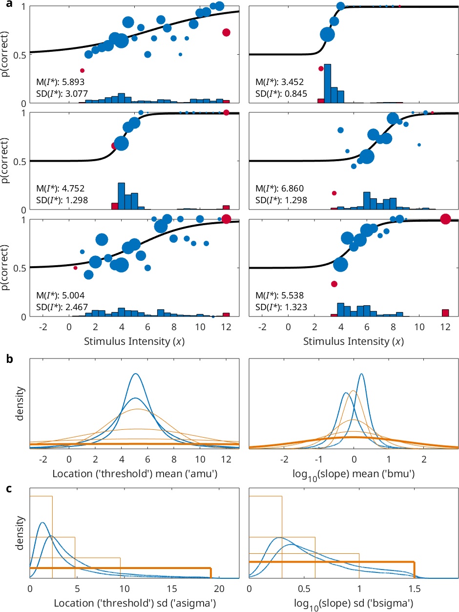 Figure 2. See text for details.
In order to determine the values for the priors' parameters, for each subject/condition combination the mean and sd of the stimulus intensities is computed (again, intensities are trimmed by
excluding the lowest and highest intensities used). These values are given in the plots in Figure 2a. The mean of the prior for the location parameters is then set to the mean of the means of
the stimulus intensities used in each condition/subject combination. In this example:
Figure 2. See text for details.
In order to determine the values for the priors' parameters, for each subject/condition combination the mean and sd of the stimulus intensities is computed (again, intensities are trimmed by
excluding the lowest and highest intensities used). These values are given in the plots in Figure 2a. The mean of the prior for the location parameters is then set to the mean of the means of
the stimulus intensities used in each condition/subject combination. In this example:
 where Ms,c(x*) is the mean of the trimmed stimulus intensities for subject s, condition c and S and C are the total number of subjects
and conditions, respectively, in the analysis.
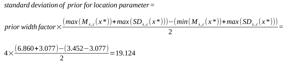
The standard deviation of the prior for the location parameter is set to the default location prior width factor (i.e., 4) times half the distance between the highest obtained mean plus
the highest obtained standard deviation and the lowest obtained mean minus the highest obtained standard deviation. In this example:
where Ms,c(x*) is the mean of the trimmed stimulus intensities for subject s, condition c and S and C are the total number of subjects
and conditions, respectively, in the analysis.
The standard deviation of the prior for the location parameter is set to the default location prior width factor (i.e., 4) times half the distance between the highest obtained mean plus
the highest obtained standard deviation and the lowest obtained mean minus the highest obtained standard deviation. In this example:
 The resulting default prior distribution is shown by the thick orange curve in the left panel of Figure 2b. The light orange curves show the prior distributions for location prior width
factors of .5, 1, and 2. In case there is only a single subject, this prior will be applied to the location parameters for each condition of that single subject. In case there are multiple
subjects included in the analysis (as is the case in the example here), the prior will be applied to the hyper parameter for the location mean ('amu') for each condition. The blue curves
show the posterior distributions for the two hyper parameters (one for each condition) for the location mean that resulted when the default prior was used. It is clear here again that the
default prior is not very informative.
In the case of multiple subjects, we also need a prior for the hyper parameter for the location standard deviation ('asigma'). The default form of the prior for this parameter is the
uniform distribution. The lower bound for the uniform distribution will be set to 0, while the upper bound will be set to the same value that is used for the standard deviation of the
prior for the location parameter (here: 19.124). The uniform distribution shown in thick orange lines in the left panel of Figure 2c corresponds to the default prior for the standard
deviation of the hyper parameter for the standard deviation of the location parameters. The lighter orange curves show the priors when the location prior width factor is set to
.5, 1, or 2.
The prior for the log10(slope) parameter is chosen as in the case for a single PF except that now it is based on the average standard deviation of the trimmed stimulus intensities.
Here, the average standard deviation equals:
The resulting default prior distribution is shown by the thick orange curve in the left panel of Figure 2b. The light orange curves show the prior distributions for location prior width
factors of .5, 1, and 2. In case there is only a single subject, this prior will be applied to the location parameters for each condition of that single subject. In case there are multiple
subjects included in the analysis (as is the case in the example here), the prior will be applied to the hyper parameter for the location mean ('amu') for each condition. The blue curves
show the posterior distributions for the two hyper parameters (one for each condition) for the location mean that resulted when the default prior was used. It is clear here again that the
default prior is not very informative.
In the case of multiple subjects, we also need a prior for the hyper parameter for the location standard deviation ('asigma'). The default form of the prior for this parameter is the
uniform distribution. The lower bound for the uniform distribution will be set to 0, while the upper bound will be set to the same value that is used for the standard deviation of the
prior for the location parameter (here: 19.124). The uniform distribution shown in thick orange lines in the left panel of Figure 2c corresponds to the default prior for the standard
deviation of the hyper parameter for the standard deviation of the location parameters. The lighter orange curves show the priors when the location prior width factor is set to
.5, 1, or 2.
The prior for the log10(slope) parameter is chosen as in the case for a single PF except that now it is based on the average standard deviation of the trimmed stimulus intensities.
Here, the average standard deviation equals:
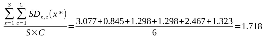 Thus the mean for the prior on log10(slope) values is set to 1.718. The standard deviation of the prior for log10(slope) values is again set to the default prior width factor
of 1.5. When only one subject is included in analysis these values are applied to the priors for the log10(slope) values in all conditions. When more than one subject is included
in the analysis, the mean and standard deviation values are applied to the priors for the hyper parameters corresponding to the mean log10(slope) value ('bmu') across subjects for
each condition.
In the case of multiple subjects, we also need a prior for the hyper parameter for the log10(slope) standard deviation ('bsigma'). The default form of the prior for this
parameter is the uniform distribution. The lower bound for the uniform distribution will be set to 0, while the upper bound will be set to the default value for the slope's
prior width factor. The uniform distribution shown in thick orange lines in the right panel of Figure 2c corresponds to the default prior for the standard deviation
of the hyper parameter for the standard deviation of the log10(slope) parameter. The lighter orange curves show the priors when the prior width factor is set to .5, 1, or 2.
In case a custom model matrix (see www.palamedestoolbox.org/modelmatrix.html) is supplied, the priors for the parameters that the model matrix defines (which we refer to as
reparameters) are determined as above but should be appropriately scaled as explained below. As an example, let's say that in the analysis above the location and
log10(slope) parameters were reparameterized using the following model matrix:
Thus the mean for the prior on log10(slope) values is set to 1.718. The standard deviation of the prior for log10(slope) values is again set to the default prior width factor
of 1.5. When only one subject is included in analysis these values are applied to the priors for the log10(slope) values in all conditions. When more than one subject is included
in the analysis, the mean and standard deviation values are applied to the priors for the hyper parameters corresponding to the mean log10(slope) value ('bmu') across subjects for
each condition.
In the case of multiple subjects, we also need a prior for the hyper parameter for the log10(slope) standard deviation ('bsigma'). The default form of the prior for this
parameter is the uniform distribution. The lower bound for the uniform distribution will be set to 0, while the upper bound will be set to the default value for the slope's
prior width factor. The uniform distribution shown in thick orange lines in the right panel of Figure 2c corresponds to the default prior for the standard deviation
of the hyper parameter for the standard deviation of the log10(slope) parameter. The lighter orange curves show the priors when the prior width factor is set to .5, 1, or 2.
In case a custom model matrix (see www.palamedestoolbox.org/modelmatrix.html) is supplied, the priors for the parameters that the model matrix defines (which we refer to as
reparameters) are determined as above but should be appropriately scaled as explained below. As an example, let's say that in the analysis above the location and
log10(slope) parameters were reparameterized using the following model matrix:
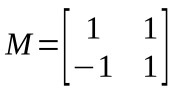 The first row defines a reparameter that corresponds to the sum across conditions, the second defines a parameter that corresponds to the difference between conditions.
Above we argued that based on stimulus placement, a value of 5.250 would be a relatively likely value for each of the two location hyper parameters (one for each condition)
and thus we center the priors for each condition on that value. However, if the above model matrix is used, the first reparameter corresponds to the sum of the location
parameters in the two conditions. The result is comparable to a rescaling of the stimulus intensities by a factor equal to the sum of the coefficients. Of course, when we rescale
a dataset by a multiplicative factor, the mean of the dataset scales by the same multiplicative factor. For example, it is easy to see that if a value of 5.250 is a likely value
for the location in each condition, a value of 2 x 5.250 = 10.500 would be a
likely value for the sum of the location parameters in the two conditions. Generally, the value for the mean of a prior for a reparameter should be scaled by the sum of the coefficients
that define the reparameterization. Note that when we apply the same rule to the second reparameter, the prior for it will be centered on 0. Effectively, this favors
the value of 0 for any difference in the values for the parameter across conditions (i.e., it favors the hypothesis that there is no effect of the variable that is
manipulated between conditions).
The standard deviation of prior distributions, on the other hand, should be scaled by the sum of the absolute values of the coefficients defining the reparameters.
For this example, the standard deviation for the first as well as the second reparameter defined by matrix M above are scaled by a factor of 2.
The first row defines a reparameter that corresponds to the sum across conditions, the second defines a parameter that corresponds to the difference between conditions.
Above we argued that based on stimulus placement, a value of 5.250 would be a relatively likely value for each of the two location hyper parameters (one for each condition)
and thus we center the priors for each condition on that value. However, if the above model matrix is used, the first reparameter corresponds to the sum of the location
parameters in the two conditions. The result is comparable to a rescaling of the stimulus intensities by a factor equal to the sum of the coefficients. Of course, when we rescale
a dataset by a multiplicative factor, the mean of the dataset scales by the same multiplicative factor. For example, it is easy to see that if a value of 5.250 is a likely value
for the location in each condition, a value of 2 x 5.250 = 10.500 would be a
likely value for the sum of the location parameters in the two conditions. Generally, the value for the mean of a prior for a reparameter should be scaled by the sum of the coefficients
that define the reparameterization. Note that when we apply the same rule to the second reparameter, the prior for it will be centered on 0. Effectively, this favors
the value of 0 for any difference in the values for the parameter across conditions (i.e., it favors the hypothesis that there is no effect of the variable that is
manipulated between conditions).
The standard deviation of prior distributions, on the other hand, should be scaled by the sum of the absolute values of the coefficients defining the reparameters.
For this example, the standard deviation for the first as well as the second reparameter defined by matrix M above are scaled by a factor of 2.